All about R mutual love
Nutshell
R is an object-oriented, functional, vectorized scripting language designed for statistics. Object-oriented refers to the objects taken and returned by functions from which quantities are strategically extracted (contrast this against SAS or SPSS which simply ‘spit out’ output). Functional refers to R’s strong reliance on functions, from the most complex statistical methods to simple base operators. Vectorized refers to vectors being the central data structure in R (contrast this against Matlab’s preference for matrices), playing a key role in the speed of functions.
This free, open-source software facilitates all major aspects of data analysis, and serves as a home for most methodological development in statistics and machine-learning; making it an exceptional programming language for analysts, statisticians, and data scientists.

Settings
First off, install R and RStudio according to your OS (many existing resources). RStudio offers an intutive yet powerful interface for R, making it a great front-end. Fortunately most of RStudio’s default settings are very useful like autocomplete, syntax highlighting, and certain shortcuts, so its great out-of-the-box. Settings may be accessed by choosing Tools -> Global Options in the control panel. Some additional settings making day-to-day programming more enjoyable for me are:
- Pane Layout - arrange the four windows into a format that pleases you. Personally I prefer the source in top-left, console top-right, environment bottom-left, and help bottom-right.
- General - uncheck the “Restore .RData file”, as it may cause a longer load-time depending on the previous environment.
- Appearance - choose an editor theme that suits your taste.
Disclaimer: We restrict ourselves to rectangular data (i.e. columns are variables, rows are individual observations) throughout this entire document for simplicity.
Mechanics
Some understanding of R’s underlying mechanics can exponentially improve the skill of any programmer. Below I address three crucial, technical aspects of R: data structures, data modes, and functional programming. Throughout each section I include relevant functions worth cataloguing for future reference.
Data Structures
Data is contained within a certain structure in one or more modes or variable types according to the structure. The essential structures are scalars, vectors, matrices, arrays, lists, and data frames. With the exception of lists and data frames, all elements in a vector must be of the same mode. Below we’ll see that data structures may be conceptualized as modified vectors of some sort, with certain restrictions on the modes of the vectors it contains.
Vector
The atomic data structure in R of which all others are composed, and the structure most functions are optimized to operate on. All elements in a vector must be of the same mode. Elements are stored contiguously in a vector, and require no explicit declaration of the pointer or its mode unlike Java or C. Three key ideas we’ll illustrate below are recycling (automatic lengthening of vectors), filtering (extraction of vector elements meeting certain conditions), and vectorized operations (function applied to vector is actually applied element-wise to the vector).
#valid declarations
x <- c(2,3,4)
y <- c(T,F,F,T,F)
z <- vector(length = 1, mode="integer")
z[1] <- 3L

#query properties of vector
typeof(z)
length(x)

#vector arithmetic + recycling
x + 2
x / z

#filtering
x[x > z]   #recycling and vectorization of '>' operator.
y[c(2,4,5)]
x[-c(1:2)]
subset(c(2,3,NA,4),c(2,3,NA,4)>2) #differs from [] by handling of NA values
seq() - returns a sequence of numbers of a certain length, or in a given range.
rep() - returns a vector repeating some shorter vector.
all()/any() - returns T or F for whether all/any elements in a vector satisfy some logical condition.
which() - returns a vector containing the positions of elements within the inputted vector satisfying some logical condition.
ifelse() - returns a vector of equal length where each element is one inputted value if some logical condition is satisfied, else it is another inputted value.
summary() - returns median, minimum, maximum, and other quantile information of a vector.
Scalar
A one-element vector for all intents and purposes.
Matrix
Collection of vectors, all of the same mode, or more technically a vector with two additional attributes: number of rows and columns. Elements are stored in column-major order. Indexing or filtering can become quite complex, especially when done simultaneously on rows and columns, but may conveniently extract vectors or submatrices.
#valid declarations
x <- matrix(c(1,2,3,4),nrow=2,ncol=2)
y <- matrix(nrow=2,ncol=2)
y[1,1] <- 5
y[2,1] <- 6
y[1,2] <- 7
y[2,2] <- 8
z <- matrix(c(2,2,4,4,6,6),nrow=2)

#query matrix class
class(x)
attributes(x)
typeof(x)

#matrix arithmetic and linear algebra
x*y
x%*%z
x-y
x*2

#filtering
z[,1:2]
z[1,1:2]
z[,z[2,] >= 4] #complex, think carefully about this.

#matrix reassignment
xy <- cbind(x,y)
z1 <- rbind(z,1)
colnames(xy) <- c("eenie","meenie","miny","moe")
rownames(xy) <- c("catch","tiger")ncol()/nrow() - returns the number of rows or columns in a matrix.
cbind()/rbind() - binds vectors together by columns or rows.
x[,,drop=F] - retains the matrix status of the data, otherwise downgraded to a vector.
apply() - key function in R for which there exists a family of functions.
Array
Stack of matrices, where each matrix may be of a different mode. Multi-dimensional arrays may be created by combining multiple arrays.
#declarations, properties, filtering
z <- array(data=c(x,y),dim=c(2,2,2)) #dim=c(rows,columns,layers)
attributes(z)
z[1,2,2]
List
Recursive vector, where each element may contain any other data structure including a list. Between elements there may be different modes, but within elements mode must be same unless element is a list. Fundamental data type of most complex output in R.
#valid declarations
x <- list(name = "Donald", salary = "400000", politics=T) #tags(e.g. name) are optional
y <- vector(mode = "list") #list is technically a vector

#list reassignment
y$a <- c(T,F,T) #adding an element
y[2:5] <- c("testing", "1", "2", "3") #single brackets can access multiple items
y[[6]] <- x #double brackets access individual elements; recursion of lists
y$a <- NULL #deleting an item
lapply() - apply function where the input and output are lists.
sapply() - apply function where the input is a list and output is a matrix.
unlist() - reverts each element in a list to the least common denominator, where list with any recursion are collapsed into a vector.
Data frame
Matrix-like lists, where each column (element) may be of a different mode, but must be of the same length. Tibbles are modified data frames differing in how they print and subset, and optimized for use with the tidyverse collection of packages.
#valid declarations
superhero <- c("Batman", "Robin")
age <- c(34, 16)
z <- data.frame(superhero, age, stringsAsFactors = F)

#query structure
str(z)
names(z)
dim(z)

#accessing and filtering elements
z[z$age<18,] #access like matrix while filtering with list accessing
z[[1]][1] #access like a list
z[,1,drop=F] #retains column as data frame

#Useful functions: merge(), complete.cases()
z <- rbind(z, list("Flash", 22))
z$universe <- rep("DC", 3)
z2 <- rbind(z[c(1,3),], list("Hulk", 31, "Marvel"))
z2$sex <- rep("M",3)
merge() - matches columns of different names containing the same.
complete.cases() - returns the rows where all values are not missing.
Data Modes
The essential modes of any data are integers (int), doubles/numeric (dbl, floating-point numbers), characters/strings (chr), logical/Boolean (lgl), factors (fctr), and date-times (dttm). Cumulatively, these modes correspond to the large majority of variable types one is likely to encounter.
Integers
e.g. -1,0,1,…; subject to all of R’s typical commands.
celing()/floor() - rounds up or down to the nearest integer.
as.int() - converts vector into an integer.
Doubles
e.g. -1,0,1.354,…; subject to all of R’s typical commands; FlOP’s (floating point operations) are something to be wary of when numerical precision is an issue.
Strings
e.g. “test string”, “/uOOb5”; when combined with regexps (regular expressions: a terse language describing common patterns in strings) and the stringr package, strings are instrumental in manipulating structured and unstructured data.
#Mechanics
x <- "Valid string declaration"
y <- 'Also a "valid" declaration' #single quote allows quotes inside a string
z <- c("these", "are", "elements", "a", "string", "vector.")
?"'" #returns a complete list of special characters
Note: all of the following functions are from the stringr _ package, which avoids most of the inconsistencies in base R’s string methods._
regex() - controls finer details of string matching; all str_.() functions are automatically wrapped into a regex() call.
str_length() - returns the number of characters in a string.
writeLines() - returns string with translated escape characters; regular print prints raw contents.
str_c() - combines two or more vectors of strings at the element-level; sep= option defines the character separating tuple-wise concatenations, collapse() option further concatenates tuple-wise concatenations into a single vector.
str_split() - splits a string into pieces by inputted character.
str_view() - returns illustration of the first match in a string; requires htmlwidgets package; anchors ^ $ match beginning and end of string respectively, both match complete string; str_view_all() returns illustration of all matches in a string; character classes and alternatives facilitate matching; number of matches may be controlled through ?, +, and * (0-1, 1 or more, 0 or more).
str_extract() - returns first extracted matching piece of string element; str_subset() returns subset of string vector containing matches; str_extract_all() returns all matches in a string element if they exist; str_match() returns matches in a matrix.
str_sub() - extracts parts of a string corresponding to inputted first and last position;str_locate() returns starting and end position of every match.
str_detect() - returns equal-sized logical vector, TRUE if match is found; str_count() returns the number of matches in each string.
str_replace() - replaces exact matches in a string with new strings; str_replace_all() enables multiple repalcements.
Logical
e.g. T, F; some useful operators and functions are:
<, <=, >, >=, ==, != - less than, less than or equal to, greater than, greater than or equal to, equal to, not equal to.
!x, x|y, x&y - negates x, inclusive or, and.
%%, %/% - modular arithmetic, integer division.
if(), else(), while() - three fundamental control statements.
ifelse() - vectorized if-else.
Factors
Correspond to categorical or nominal variables; advantageous to strings when there exist a fixed number of categories, and when sorting other than ABC order is required; characters internally coded by levels; levels cannot be snuck in without previous programming;
xf <- as.factor(c(8,3,8,5))
str(xf)
unclass(xf)
attr(xf,"levels")

x1 <- c("Dec","Apr","Jan","Mar")
month_levels <- c("Jan","Feb","Mar","Apr","May","Jun","Jul","Aug","Sep","Oct","Nov","Dec")
y1 <- factor(x1, levels = month_levels)
tapply() - applies function onto sub-groups of the input vector, where groups are defined by a list of one or more factors.
split() - splits data into groups as in tapply().
by() - applies a function separately to a date frame where observations are split by factors.
aggregate() - applies a function to columns in grouped data frames defined by factors.
table() - creates one, two, and three-way contingency tables based on factors; subtable() for subtable extraction.
cut() - generates factors by binning doubles or integers into semi-open categories.
The following functions require the forcats package:
fct_recode() - changes the value of each factor level, or combines various levels.
fct_collapse() - collapses many factor levels into a small number of levels.
Date-Times
Three types of date/time objects exist: dates, times, and date-times; many packages exist in R for date-times, we focus on the lubridate package.
#Mechanics
#parse date-times from existing strings
ymd("2017-01-31")
ymd("20170131")
mdy("January 31st, 2017")
dmy("31-Jan-2017")

ymd_hms("2017-01-31 20:11:59")
mdy_hm("January 31st, 2017 8:01pm")

#from individual components in columns
flights %>%
  select(year, month, day, hour, minute) %>%
  mutate(
    departure = make_datetime(year, month, day, hour, minute)
  )
#between types
as_datetime(today())
as_date(now())
Accessors() - pull out individual parts of the date-time or reassign components of date-time, e.g. year(), month(), day(), mday(), wday(), hour(), minute(); label=TRUE provides names for the appropriate components; update(), allows reassignment of multiple parts of a date-time.
rounding() - rounds date to nearby unit of time, e.g. floor_date(), round_date(), celing_date().
durations() - represents date-time in exact number of seconds, i.e. physical time, useful for arithmetic, e.g. dseconds(), dminutes(), dhours(), ddays(), dweeks(), dyears(); unexpected results may occur with DST, leap years, etc.
periods() - represent date-time in an intuitive, human time, arithmetic also works; seconds(), minutes(), hours(), days(), week(), years().
intervals() - useful in determining the length of a span in human time.
Functional Programming
Functions play a unique role within R, and are useful in automating recurring tasks in a powerful way. All functions have three components: a name, arguments, and a body. One suggestion for readable code is to use a descriptive verb for the name, and nouns for the arguments. Arguments usually supply data as the first parameter, along with all other function-specific settings in the other parameters. Another suggestion is to use comments through ‘#’ to describe the “why” of the code, and revise the code such that the “what” and “how” are discernable with minimal effort. After creating a function in R, we are free to use it as we would any other:
illustrate_suggestions <- function(data=y, param1=p1, param2=p2){

  #Here we would describe the first crucial step of this function
  print("Really great stuff would happen here, primarily modifying y")
  local_variable <- y+p1+p2
  #
  #
  #
  #Until we finaly finished our task
  print("Last crucial step")
  local variable
}
In-built error checks created through ad-hoc testing of your functions help make your function more robust. For more serious, package-quality functions, ad-hoc testing of the function may be formalized through unit testing. Some unique properties of functions that are worth discussing are that functions are themselves objects, so they can be used as such. Related to the objects, R’s functions are polymorphic, meaning that the same function call leads to different operations for objects of different classes. For you, that means you memorize one function (e.g. plot()) to handle many different objects. Lazy evaluation is another property wherein an expression within a function isn’t evaluated until absolutely necessary. Usually, the last quantity returned by a function is the last statement evaluated, but you can make it explicit at your convenience through a return(), such as when you’d like to highlight a simpler solution. Lastly, generally speaking variables within a function are local variables (i.e. only exist within the function), while global variables exist outside a function in what is called the global environment.
Day-to-day Analysis
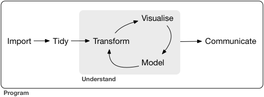
With some of the underlying mechanics of R at our disposal, we may now illustrate some practical, everday tools for your workflow. Generally speaking most of your time spent programming is comprised of importing data and cleaning it (i.e. tidying it). Then, depending on how much subject expertise and context you understand and pre-planning you’ve done, you might iterate through feature engineering (i.e. tranform), visualizing data to gain intuition and solidify insight, and perform some analysis most likely involving a model; after which you would communicate the results:
For the second half of this summary, we’ll outline the goal of each step in this pipeline, along with some key ancillary functions.
Importing Data
Reading in data is the first step in any analysis. Our focus is on the readr package given its speed (~10x faster), the fact that it defaults to a tibble, and reproducibility (won’t inherit local OS behavior). Additionally, we focus on CSV files since they are the most common form of data storage.
read_csv - reads in csv files and individually parses each column by using the first 1000 rows to guess the type of vector through guess_parser(), and using that guess to parse the column through parse_guess(); skip = n options skips the first lines of a data file, e.g. meta-data; comment = “#” drops all rows starting with the user-inputted character; na = “” specifies what value(s) represent missing values; col_types = e.g. cols(x=col_double, y=col_character) manually specificies column types (this is highly recommended); column_names takes F to input dummy column names, or a string vector for column names; read_csv2 takes semi-colon separated files, read_tsv() tab-delimited files, read_delim() files separated by any delimiter, read_fwf() fixed-width files, and read_log() Apache style log files.
Internally, read_*() depends on parsing functions, of which there exist one for every data mode. parse_*() take a character vector to part for its first argument, and another specifiying which values to treat as missing.
parse_logical() - straight-forward.
parse_integer() - straight-forward.
parse_double() - numeric parser handling different ways of specifying parts of a number (e.g. decimals) through a locale() option.
parse_number() - flexible numeric parser handling doubles with non-numeric characters before or after a number (e.g. $20, 20%) and grouping characters (e.g. 1,000,000).
parse_character() - handles different ways of encoding strings, e.g. ASCII, UTF-8.
parse_factor() - handles categorical variables by requiring an additional character vector specifying the levels in the levels = option.
parse_datetime() - parses date-time in an ISO8601 format, e.g. “2010-10-01T2010”; parse_date() parses the previous component prior to “T”; parse_time() in addition to the hms package can handle military and am/pm time; locale = locale(“”) option handles different ways dates are specified internationally.
Relational Data
Often our final data set enabling us to answer our analytic questions requires assembly from multiple data sets. Collectively this disparate data is called relational data. SQL is the most important API (applied programming interface) for relational databases, but assuming we already have the data loaded into R’s memory, there exist valuable tools in R to assemble this final data set. In fact, many of useful functions for relational data are inspired by SQL’s conventions.
Ideally data sets contain variables which are either primary or foreign keys, i.e. a unique identifier for observations in its own table or another table. Sometimes variables may be both primary and foreign, and other times data may not contain any primary key, but foreign keys are always required to relate data sets. If a primary key does not exist, a surrogate key may be created to serve as the unique identifier for observations. Relations are formed by a primary key and the corresponding foreign key in a separate data set.
*_join() - mutating joins connect rows in one data set to matching rows in another, i.e. column-matching; inner keeps mutually inclusive observations, left keeps only observations in the first, right in the second, and full creates dummy observations to keep observations existing in either data set; duplicate keys in either data sets are correctly handled through multiple matching, but are likely to be incorrectly handled (Cartesian product) if duplicate keys exist in both data sets.
*_join() - filtering joins retain ( semi) or discard ( anti) observations in one data set, if they match to observations in another.
Some additional tips for using these functions is to establish a primary key, identify any observations missing or misspelled in this key, and to double-check matches to foreign keys.
Tidying Data
Tidy data is essentially data in a tibble with each variable in a column. Making data tidy upfront saves time that would otherwise be spent cycling back and forth between analyzing and reformatting data, freeing one’s attention to the analytic questions. Below are three properties which accurately describe tidy data, along with some functions useful in achieving that property:
Each variable occupies a single column.
gather()- combines multiple numeric columns under a new single variable, e.g. when column names are actually values of a separate variable (key).
unite()- combines multiple string columns under a new single variable; sep = “” controls the characters between each string.
separate()- opposite ofunite(), i.e. pulls apart a single string column into multiple columns according to a separator.Each observervation occupies a single row.
spread()- “opposite” ofgather, i.e. useful when an observation is scattered across multiple rowsEach value occupies its own cell.
Missing data requires special handling from both a statistical and programming perspective. For the purposes of tidying data, we focus on the latter. In this vein, all we need to know is that data may be missing explicitly (i.e. censored, flagged with NA) or implicitly (i.e. truncated, not present in the data).
Explicit missing data is generally represented with NA, and if implicitly missing is technically still NA although not present. If missing data exists in the data as any value other than NA, this should be handled when reading in the data. Multiple NA values exist for each mode. In programming, most functions utilize an na.rm = T option to ignore missing data, but this may be explicitly controlled. NULL on the other hand represents value which don’t exist, in contrast to values which exist but are not present. They are often useful in loops or deleting elements from a list or vector. Some useful functions for missing data besides the na.rm = option are:
complete() - finds all unique sets of of a combination of columns (typically factors) and fills remaining columns approriately with NAs.
complete.cases() - returns a boolean vector, where F captures rows with at least one NA; useful to capture observed or missing rows.
fill() - replaces NA values in the column vector of a data frame with the former (LOCF, last observation carried forward) or latter observation; useful for missing longitudinal data.
Transformation and Summaries
Often we need to reorder columns, identify a meaningful subset of observations, or create new features to name a few data challenges. For the majority of data manipulation challenges, these functions provide essential building blocks:
group_by() - changes scope of function from operating on the entire dataset to user-specified groups.
filter() - extracts observations according to specified values; excludes rows with FALSE and NA values unless explicitly preserved; helper functions are between().
arrange() - reorders rows according to specified variables.
select() - identifies and reorders variables.
mutate() - creates new variables by transforming existing ones.
summarize() - creates flexible grouped summaries when combined with group_by().
Math & Modeling
Calculus, set operations, and linear algebra are some of the fundamental tools for analysis of any sort. Here are some of the fundamental operations:
Mathematical Functions
exp() - base e exponential function.
log() - natural logarithm.
log10() - base 10 logarithm.
sqrt() - square root.
abs() - absolute value.
trig() - trigonometric functions, e.g. sin(), cos(), tan(), acos(), sinpi().
min() max() - minimum and maximum value element within a vector.
which.min() which.max() - index of minimum and maximum element within a vector.
pmin() pmax() - element-wise minima and maxima of several vectors.
sum() prod() cumsum() cumprod() - sum, product, cumulative sum, and cumulative product of elements within a vector.
round(), floor(), ceiling() - round to closest integer, round down to closest integer, round up to closest integer.
Combinatorics
factorial() - factorial function.
choose(n,k) - number of possible subsets of size k from set of size n.
combn(x,m) - generates all possible combinations of n elements in vector x, taken m at a time.
Linear Algebra
crossprod() - matrix cross product.
t() - matrix transpose.
qr() - QR decomposition.
chol() - Cholesky decomposition.
det() - matrix determinant.
eigen() - eigenvalues or eigenvectors.
diag() - extracts diagonal of a square matrix or creates a diagonal matrix.
sweep() - performs numerical analysis sweep operations.
Set Operations
union(x,y) intersect(x,y) - union and intersection of sets x and y.
setdiff(x,y) - intersection of sets x and y, i.e elements in x but not in y.
setequal(x,y) - tests for equality between x and y.
c %in% y - membership tests return a boolean, T if c is an element in vector y.
Probability & Statistics
d*() - probability distribution (density or mass) function.
p*() - cumulative distribution function.
q*() - quantiles of some distribution function.
r*() - generates random variates of some distribution.
set.seed(x) - sets the random seed to scalar x; useful for reproducible simulations.
mean(), mode(), quantiles() - certain statistics of a distribution.
See library(help = “stats”) for a complete list of models, tests, statistics and optimization procedures.
Statistical Modeling
Statistical models serve as illuminating and useful approximations to real-world phenomena. Under certain assumptions, limitations, and properties, models can capture strong signals in data in the presence of noise, effectively partitioning the data into patterns and residuals. Here is the basic modeling syntax for the linear model, and many other models in R:
model_name <- model(y~x1+x2+..., data= <DATA>)Y is generally the response or outcome, and x the continuous or categorical covariates or features which may explain the signal. Interactions between covariates and transformations of existing covariates are also valid input for the right-hand of the equation. When one of our variables is an effect modifier with many levels, it becomes imperative to apply functions from the purrr and broom packages to create many models on sub-data frames. For now we focus on the basics.
Some packages to apply other models are:
stats::glm() - generalized linear models; extends linear models to outcomes in the exponential family.
mgcv::gam() - generalized additive models; extend glms to incorporate arbitrary smooth functions on the right-hand side.
glmnet::glmnet() - extend glms to scenario where there are nuisance variables that require shrinkage or elimination by penalizing the loss function in a variety of ways.
MASS:rlm()) - robustifies the linear model to influential outliers unduly affecting inference, at the cost of decreased performance in the absence of outliers.
rpart::rpart() - i.e. tree-based methods fit a piece-wise constant model that extends gams in a theoretical sense, effectively splitting the data into rectangles for prediction; many variants exist such as random forests randomForest::randomForest() or gradient-boosted machines xgboost::xgboost.
Predictions, residuals, and general goodness-of-fit measures are all valuable in assessing the fit and value of our model. While the latter is usually provided as default output in the model, the former two many not be. One model agnostic approach to obtaining such predictions is to generate an evenly spaced grid of values covering the same region as our data and add predictions to this grid. One way of achieving this is to use modelr::data_grid() to generate all combinations of unique variables in the provided data frame, and simply use modelr::add_predictions() to add corresponding predictions.
Residuals are far easier in that we simply compute the discrepancy between our model’s prediction and the data through modelr::add_residuals(). To continue exploring patterns, we might visualize the residuals and continue modeling on the residuals until the subsequent residuals look like random noise, or equivalently all major patterns have been exhausted. One cautionary note is that as our number of variables increases, our ability to model signal in our data becomes limited by our ability to visualize models and residuals.
Visualization and Communication
Visualization is a crucial tool for exploring patterns in data and conveying meaningful insight to others. R’s generic plot() function is very powerful and well-integrated with many other base R packages, but our focus is on the ggplot2 package. Although its syntax is noticably different, the quality of the plots it produces unquestionably outshines base R plots. For that reason we focus on ggplot2.
In general, the basic syntax of ggplot is:
ggplot(data = <DATA>) +
  geom_*(mapping = aes(<MAPPINGS>),
         stat = <STAT>,
         position = <POSITION>,
         )  +
  labs()    + ...
ggplot() - creates a coordinate system that is layered on through additional geom_*() calls; mappings placed within ggplot() are global.
geom_*() - family of functions adding layers to ggplot(); core plots are point(), histogram(), boxplot(), density(), violin(), each with their own aesthetics; mappings added to geom objects are local, enabling layer-specific aesthetics and data; each geom computes a default statistic which may be overrided.
mapping = aes() - defines how variables in the data are mapped to visual properties; the mapping argument is always paired with aes(); x and y arguments of aes() specify which variables to map to the x and y-axes; color() size() alpha() or shape() differentiate between observations according to some variable, creating a legend automatically when called within the aes() call, and can be controlled manually by calling options outside the aes() call; position = alternates the placement of certain 2d plots, e.g. bar.
facet_* - separates plots into sub-plots by classes; facet_wrap makes smalls subplots for each class; nrow = controls the number rows for the subplots; facet_grid() subdivides classes within a larger plot.
coord_*() - controls the coordinate system; coord_flip() switch the x and y-axes; coord_quickmap() correctly sets the aspect ratio; coord_polar() uses polar coordinate.
labs() - layers labels on the plot; x = , y = , color = customize the appropriate labels and calling quote() within these enables mathematical notation; title = adds a title; subtitle = adds a subtitle below the title; caption = adds a caption on the bottom right.
geom_label() - adds annotations to individual observations or groups and adds rectangles to highlighted observations; geom_text() only adds text to observations; geom_label_repel improves geom_label() by preventing overlapping labels.
scale_*() - controls axis ticks and legend keys; mode-specific.
theme() - controls non-data parts of plot, e.g. legend.
coord_cartesian() - enables zooming in on regions of the plot.
A couple of general tips for creating effective visualizations are to convey one or two points simply and elegantly (viewer shouldn’t have to think too much to ‘get it’), where the aesthetics support rather than overshadow the key information. One great tool for quick exploratory visualizations of data is through the esquisse:::esquisser() command, which is accessible as an addin in RStudio after installing esquisse. For a masterclass of some potential visualizations using ggplot2, another highly recommended source is Selva’s post on RStatistics.
To prepare formal documents with embedded code, both Sweave and Markdown are integrated within RStudio for ease of access. Many existing resources exist to choose between them and learn how they work, but personally I prefer RMarkdown.
Coda
R is free, R is open-source, and with a little practice, R may assist you in cracking open meaningful questions by probing data. Together with the tidyverse, R is one of the first languages designed to enable the writing of intuitive, readable code, which promotes collaboration and reproducibility. Ultimately, it is not about what language you speak (or code), but about the insight you may convey through that language. R is not only a medium to convey such insight, but a laboratory wherein one may make the requisite discoveries. All of this and more is possible with a laptop, some ingenuity, and lots of coffee.
Lick the Spoon
Cheatsheets - For many of the important packages discussed above, along with some others we haven’t, R helps you stay ahead of the curb: https://www.rstudio.com/resources/cheatsheets/
Performance - Regardless of the individual capacities of one’s individual CPU, speed and memory will always be limited by R’s preferred programming styles and memory allocation procedures. Speed is often an issue for large-scale batch programs, recurring analyses, simulations, or commercial applications. The most fool-proof way to improve speed in R is simply to vectorize all applicable parts of one’s code. Three other important ways to speed up code are to allocate memory up-front instead of within a loop, rewrite CPU-intensive portions in C, C++, or byte-code, and rewrite code in parallel. Finding bottlenecks in code can be facilitated by microbenchmark for comparing small expressions, rbenchmark for code blocks and parallelized code, and Rprof() together with summaryRprof() for comparing code-blocks or functions operation by operation.
Issues surrounding R’s memory usage affect and may even halt performance altogether if the object exceeds 2^31 bytes, even on 64-bit machines with a lot of RAM. Most objects in R are immutable, thus any alteration of an existing vector results in the entire vector being recomputed. Consequently, it is worth being mindful of the reassignment or copy of any vector. When an object cannot be loaded, one intuitive approach is to chunk in the read-in of the object, i.e. to read rows of a large files utilizing the skip = n and nmax = option in the readr package, or read individual files in separately and put-off combining unless absolutely necessary. Many model estimators are not distinct from their distributed counterparts, so often it is not necessary to combine the data at all. Should we need to read in a large data-frame exceeding R’s capacities, then some worthwhile resources are the RMySQL, ff, and bigmemory packages. While performance issues are often unpredictable, the above advice together with an understanding of the some basic issues R faces should provide higher-performing code.
Parallel - When run in parallel, it is very possible that already slow code may actually become slower in R due to overhead, i.e. time wasted in noncomputational activity such as registering a cluster or manager to worker communication. Speedup may be pronounced mostly for operations which are already “embarassingly parallel”, so parallel should be used mostly for these applications, and very large-scale recurring applications when additional speed is required. Parallel code may be utilized in a multi-core machine (each core is a worker), a networked systems of computers (e.g. HTCondor or any grid), or through a high-performing GPU on a CPU (see gputools::gpuSolve(). Packages to parallelize code in R are OS specific, so generally speaking, the snow and parallel packages are useful for MacOS and foreach, doSNOW, and doParallel packages for Windows. Parallelizing code is very problem-specific, but a general strategy is to identify major bottlenecks, improve code or parallelize it, and iterate until necessary.
Interfacing - Although they require some effort, there exist packages to call other programs within R and vice-versa. Even when documenting through Markdown or StatWeave, one may embed code chunks utilizing a specific language that is not R.
Shortcuts - option-shift-K provides the shortcut to the shortcut menu, from which one may access all shortcuts.