Learn deepR: Deep Learning in R
Nutshell
Deep learning refers to a subfield of machine learning (itself a subfield of AI) that is characterized by successive layers of increasingly meaningful representations. Often these layered representations are learned via neural networks that are literally stacked on one another, or more generally connected to each other somehow (p.8 of @dl). Most of the justly deserved hype around deep learning can be traced back to a few remarkable and unprecedented breakthroughs in speech recognition and image classification which rivaled or even surpassed human abilities (p. 294 of @dl).

In some sense, deep learning is predicated on the idea that high-level features of most natural signals in images and speech can be expressed in terms of lower-level, learnable features. For example, we can imagine a cat as an image satisfying a certain “feline-profile” consisting of whiskers, cat-ears, a tail, etc. In this light, deep learning models serve as multi-stage information-distillation pipelines, where successive filters progressively increase the model’s relevance with respect to the objective of some task.
In the coming document we provide the mathematical and computational basis of deep learning, introduce certain key architectures, and provide certain illustrative examples. For those looking to improve their technique in deep learning, we briefly explain some useful skills at the very end.
Mechanics
Algorithmic advances (e.g. backpropogation), large-amounts of freely available data, highly parallelized hardware (e.g. NVIDIA GPUs, AWS, Google Cloud), and complex software (CUDA language, TensorFlow framework, Keras API) are the key technologies which enabled the flurry of successes in deep learning. Just as important are the ideas which gave rise to these models, which we will now discuss from their most basic mathematical building blocks.
Mathematics
Deep learning is often called a black-box for its complexity which prevent any useful easy interpretaton of the model. Despite this, modern models have been developed on more readily understood mathematical models or operations, the most relevant being neural networks, which we’ll discuss in addition to convolutions which underpin CNNs.
Neural Network
Neural networks have retained their mystery as they’ve evolved to encompass a large class of methods in deep learning, but here we illustrate the most simple neural network: a densely connected classifier implemented through layer_dense with an output layer.
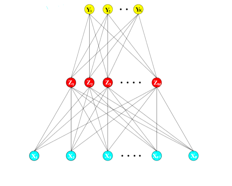
Statistically, a neural network essentially derives features \(Z_m\) from a nonlinear function of a linear combination of the inputs \(X\) in the dense layer. In the output layer, more linear combination of these derived features \(Z_m\) are taken as outputs or targets \(T_k\), and the final output \(Y_k\) is finally modeled as a function of the input \(f_k(X)\) through some function of the targets \(g_k(T)\). In mathematical terms:
\[ Z_m = \sigma(\alpha_{0m} + \alpha^T_mX), m = 1,...,M, \quad \text{dense layer} \\ T_k = \beta_{0k} + \beta_k^TZ, k = 1,...,K, \quad \text{output layer} \\ Y_k = f_k(X) = g_k(T), k = 1,...,K,\quad \text{final transformed outputs} \]
where \(Z = (Z_1, Z_2,...,Z_m)\) and \(T= (T_1, T_2,...,T_k)\). The activation function \(\sigma(v)\) is usually chosen to be the rectified linear unit, i.e. relu \(\sigma(v) =v^+ = max(0,v)\), and the activation of the output layer \(g(v)\) often depends on the problem. In case of regression an identity function is chosen \(Y_k = g_k(T) = T_k\), but for classifcation a popular activation function is the softmax function \(Y_k = g_k(T) = \frac{e^{T_k}}{\sum_{l =1}^Ke^{T_l}}\), which is the same transformation used in multicategory logistic regression. \(\alpha\) and \(\beta\) are all estimated since they are the parameters, and bias vectors \(\alpha_0\) and \(\beta_0\) are often additionally modeled. Putting it all together, we may say that:
\[ Y_k = f_{k}(X) = g_k(\beta_{0k} + \beta_k^T(\sigma(\alpha_{0m} + \alpha_m^TX))) \]
where \(\alpha\) and \(\beta\) are usually just taken to be a set of weights \(W\) which must be estimated. To better understand this simple neural network, we present a diagram below with the model we just described. The first blue layer is the input layer, the second red layer consists of the derived features, and the last yellow layer of the transformed outputs.
As we introduce different architectures, layer types, regularization techniques, and ways to connect or disconnect the layers in later sections, it should be kept in mind that this is the primary element in each model. Much of the flexibility found in later models begins here (@esl).
Convolutions
Convolution refers to a mathematical operation on two functions expressing how the shape of one is modified by the other. More precisely, it is defined as the integral of the product of two functions after one is reversed and shifted:
\[ (f*g)(t) \equiv \int_{-\infty}^{\infty}f(\tau)g(t- \tau)d \tau \]
In CNNs, the idea is to apply multiple cascaded convolutional kernels or filters onto the entire area of an input image in an attempt to construct feature maps useful in some task. To make the idea of convolution more intuitive, consider the following example from (pg 92 of @fdl), where we apply two filters to create two new feature maps. Each filter represents a potential feature, e.g. vertical or horizontal edges. Each shaded element in our output maps essentially indicates when there is a “match” between the feature captured in the filter, and the area the filter is applied on the input image.
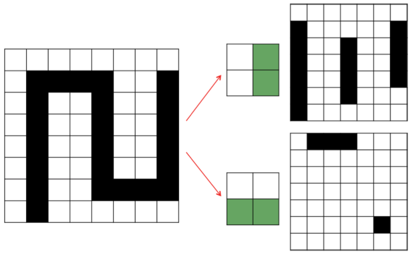
Essentially this is what happens in a convolutional layer of a deep learning model. Here are a few key differences that should help bridge the gap between this toy example, and a real CNN:
- Each element of the filter map is a single parameter that is learned by the model, so this notion of “matching” doesn’t extend too far.
- After convoluting the filters onto the input image, the resulting feature maps are passed through an activation function.
- “Input images” are only images in the first layer, after which they are filters passed through activation functions from previous layers.
- Filters are not only applied solely on a single feature map; they operate on the entire volume of feature maps that have been generated at a particular layer.
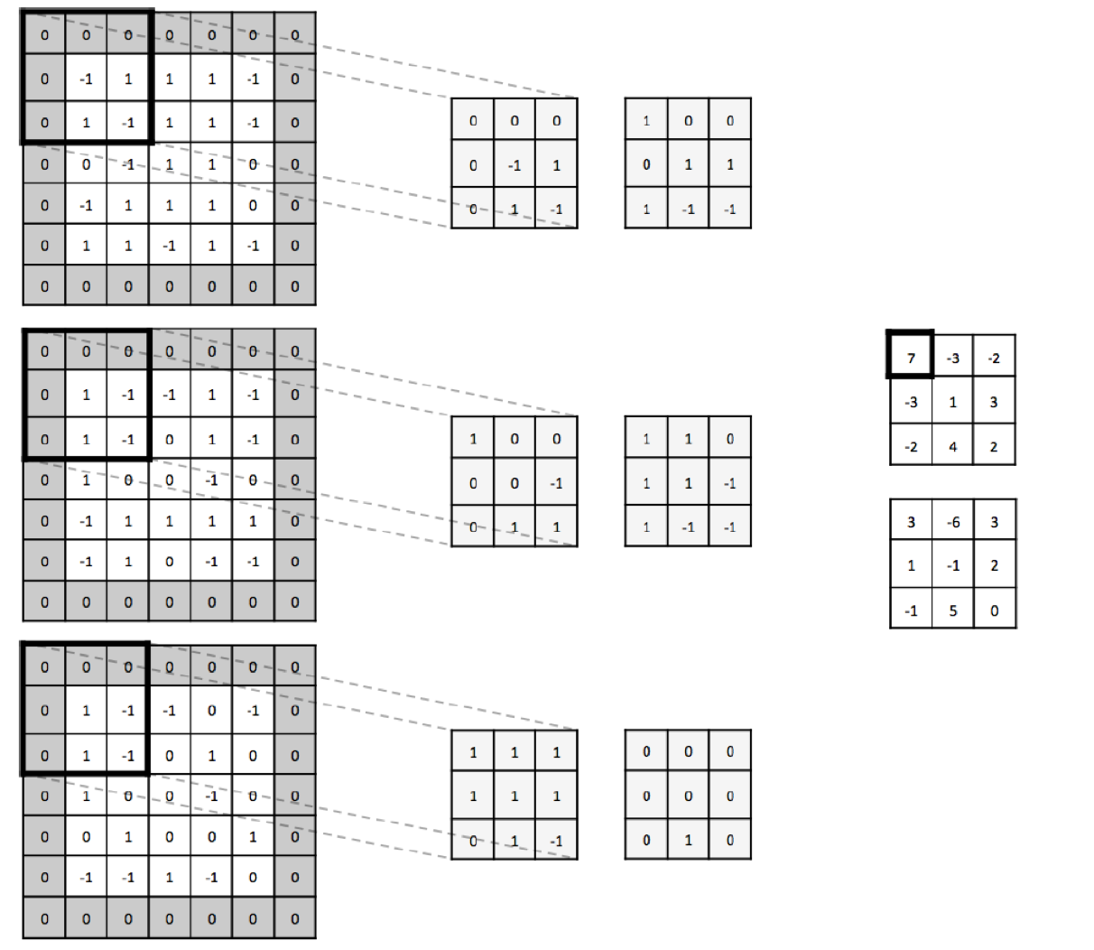
While these details increase the complexity of what is happening within a CNN, the simple fact that each filter serves as feature detectors (with more general features earlier on and more abstract task-specific features later on) still holds. To provide a more mathematical example, consider the example below where we apply a dot product (each element multiplied by each element) between the input image and the filters. The sum of those 27 multiplications result in the element in the feature map being 7.
In sum, convolutions are a useful tool which help the CNN construct features maps relevant to some task, while also helping the model scale its number of parameters as we’ll see later when we return to the code of convolutional layers.
Fitting algorithm
In the world of deep learning, one algorithm stands above all, since it was the first used to fit a successful deep learning model in 1989, and continues to be used 30 years later in some way or form: backpropagation. For brevity, we’ll just mention taht backpropogation start with the final loss value and works backwards from the top layers to the bottom layeres, applying the chain rule to compute the each parameter’s contribution to the loss, with the aid of SGD. Algorithimically, SGD is no different than any other model fitting algorithm, and we’ll focus on it now:
- Draw a batch of training smples \(x\) and outcomes \(y\).
- Apply the current model on input x (a forward pass) to obtain
y_pred.
- Compute the loss of the model on the current batch (loss measures the mismatch betwen y and x).
- Update all of the weights of the network to reduce the loss on that batch and start again.
While the overall end-goal is to get a highly predictive, generalizable model, the end-goal of the model is to achieve a very low loss on the training data. Step 1 is I/O code and step 2 + 3 tensor operations. Step 4 (the update step) is the one where some ingeunuity is needed, by way of gradient descent.
The idea behind gradient descent is to move the coefficients in the opposite direction of the gradient (i.e the multidimensional derivative and derivative of a tensor operation), thus decreasing the loss. It takes advantage of the fact that all the operations in a deep learning model are differentiable, and so computes the gradient of the loss with respect to the model parameters. Ordinarily we just differentiate the loss somehow to obtain the optimal set of parameters which minimizes the loss. Given the unwieldy number of parameters common in deep learning, this approach is not feasible.
Instead, if we put together gradient descent with the general algorithm outlined above, we can finally fit a deep learning model:
- Draw a batch of training smples \(x\) and outcomes \(y\).
- Apply the current model on input x (a forward pass) to obtain
y_pred.
- Compute the loss of the model on the current batch (loss measures the mismatch betwen y and x).
- Compute the gradient of the loss with respect to the network’s parameters (the backward pass).
- Move the parameters a little in the opposite direction of the gradient in hopes of slightly reducing the loss.
What we just described is called mini-batch stochastic gradient descent. Stochastic refers to the fact that each batch of data is drawn at random, and mini-batch to the fact that we draw batches of data. True SGD would take one observation at a time, and the extreme called batch SGD takes all of the data at each step (very costly). At the very basic, these are the ideas needed to understand the fitting algorithm implemented here for deep learning. Some other ideas worth knowing about are backpropogation and momentum, but for now we refer you to consult section 2.4 @dl for more detail.
Architectures / Problems
Deep learning architectures refer to the network of combined layers which make up a single deep learning model. Each layer is ordinarily a neural network. At its simplest, a deep learning model is a directed, acyclic graph of layers, such as a linear stack of layers. For more complex problems, the architectures tend to increase in complexity; some popular ones being two-branch networks, multihead networks, and inception blocks (p.53). Complexity is often introduced into an architecture through configuring model hyperparameters, which for deep learning are the number, size, ordering, types, and connections of layers. To illustrate the large variety of established networks consider the image below.
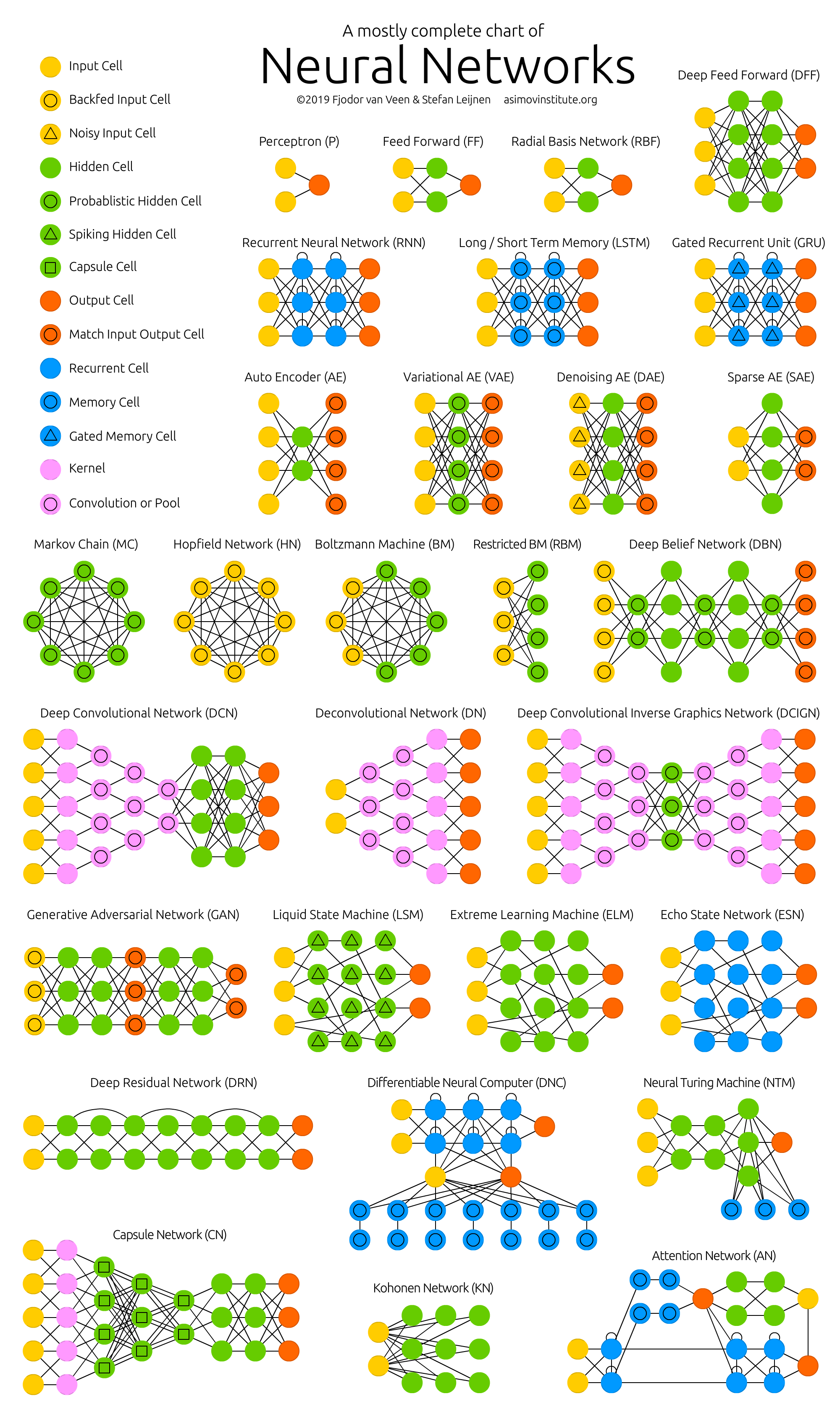
Picking a useful architecture (i.e. optimizing the hyperparameters) for a deep learning model is more of an art than a science, and for better or worse is usually driven by previous successes (p. 245 of @dl). While there is a great diversity within both of these problems, the overwhelming trend is that CNNs perform well on tasks involving visual data, while a variant of RNNs such as LSTMs or GRUs perform well on tasks where the data is sequential. While the architectures for these tend to be different, the workflow for developing the models tend to be very similar to any machine-learning workflow, with the exception of the data processing and model-building stage.
The traditional workflow for building a deep learning model is as follows:
- Process the data into tensors of appropriate shape.
- Define the deep learning network layer, by layer, where input layer takes tensors of shape equivalent to the input, and the output layer returns data of shape appropriate to the problem.
- Define the problem logistics in the compilation step, e.g. the optimization algorithm, the loss function, and the validation metric.
- Fit the model using training data and labels.
- Evaluate the data on unseen data.
#processing data into tensors of shape n*784
library(keras)
mnist <- dataset_mnist()
train_images <- mnist$train$x
train_labels <- mnist$train$y
test_images <- mnist$test$x
test_labels <- mnist$test$y

train_images <- array_reshape(train_images, c(60000, 28 * 28))
train_images <- train_images / 255
test_images <- array_reshape(test_images, c(10000, 28 * 28))
test_images <- test_images / 255
train_labels <- to_categorical(train_labels)
test_labels <- to_categorical(test_labels)

#defining a simple network: two dense layers
model <- keras_model_sequential() %>%
  layer_dense(units = 512, activation = "relu", input_shape = c(28 * 28)) %>%
  layer_dense(units = 10, activation = "softmax")

#compilation step (defining problem logistics)
model %>% compile(
  optimizer = "rmsprop",
  loss = "categorical_crossentropy",
  metrics = c("accuracy")
)

#fitting the model
history <- model %>% fit(train_images, train_labels, epochs = 5, batch_size = 128)

#evaluating the model
results <- model %>% evaluate(test_images, test_labels, verbose = 0)
predictions <- model %>% predict_classes(test_images[1:10,])
Other more general and useful tips for deep learning models (pg. 103 + pg. 50 of @dl); define problem and assemble data, develop a common-sense baseline along with a simple model to beat that baseline.
Coding Basics
Under the Keras framework with a TensorFlow backend as implemented in the keras package in R, a deep learning model at its most basic involves two simple functions: keras_model_sequential(), layer_dense(). Here is what each of those functions does:
keras_model_sequential() - kicks off a linear stack of layers for a deep learning model; its two arguments are a list of layers which may be added one after another using tidy semantics (i.e.layer() %>% layer()), and an optional name for the model.
layer_dense() - implements a densely-connected neural network; heuristically the operation this layer performs is output = activation(dot(input, weights)) + bias), where activation applies the activation funtion element-wise, specified through the activation argument, bias is an optional vector that can be estimated, it is added to the dot product by setting use_bias to TRUE. Many options exist such as weight and bias initialization, regularization, and batch sizes.
Below we specify a simple neural network model to better explain what is needed for it to work:
model <- keras_model_sequential() %>%
  layer_dense(units = 512, activation = "relu", input_shape = c(28 * 28)) %>%
  layer_dense(units = 10, activation = "softmax")
summary(model)
## Model: "sequential"
## ________________________________________________________________________________
## Layer (type) Output Shape Param #
## ================================================================================
## dense (Dense) (None, 512) 401920
## ________________________________________________________________________________
## dense_1 (Dense) (None, 10) 5130
## ================================================================================
## Total params: 407,050
## Trainable params: 407,050
## Non-trainable params: 0
## ________________________________________________________________________________Mathematically said, the model above is equivalent to:
\[ f(W_1, W_2, w_1, w_2) = g_2(W_2^T[g_1(W_1^TX^T + w_1)]^T + w_2) \] where \(\underset{60000 \times 28^2}{X}\), \(\underset{28^2 \times 512}{W}\), \(\underset{512 \times 1}{w_1}\). Although the data here is represented as whole, deep-learning models typically do not process an entire dataset, instead they process batches of it. We obtain the parameters at each layer by adding the number of elements in the weight matrix (which is composed of the number of features put into a vector times the number of hidden units, i.e. \(28^2 \times 512 = 401408\)) with the number in the bias vector (\(512\), for a total of \(401408 + 512 = 401920\)). After reshaping the input tensor appropriately, all that’s required is to correctly input the shape of the input in the first layer, and to choose an intuitive number of hidden units (usually big to small).
To increase the complexity of a model, we add layers to it. Layers in a deep learning model represent interconnected neural networks. Contiguous layers must be compatible, i.e. the input tensor shape of the latter be the output tensor shape of the former. Luckily in keras this is all taken care of, as the layers are dynamically built to match the shape of the incoming layer (p. 52 of @dl). While there exists a dizzying variety of layer types, there are three major families of architectures which address many of the common problems: densely connected networks, convolutional networks, and recurrent networks.
Each architecture performs well on specific input modalities and carries implicit assumptions to optimize the fit of the model. To give an idea of where these families are known to excel, consider the following list:
- Vector data - densely connected nets.
- Image data - 2D convnets.
- Volumetric data - 3D convnets.
- Sequential data (sound, text, time-series) - 1D convnets or RNNs.
- Video data - 3D convnets or combo of 2D convnet with RNN / 1D convnet.
We’ll spend some time on each below.
Convolutional Layers
Convolutional layers produce a tensor of outputs by convoluting the filter or kernel onto the input tensor. In more detail, each element in each filter represents a parameter we want to learn, and each filter is a feature map, which when convoluted against the input results in a response map (p.116 of @dl). As input, convnets take input tensors of shape (image height, image width, image channels). Batch or sample size is also an input, but not directly relevant to constructing the net. The output of every layer of layer_conv_2d() and layer_pooling() is a tensor of shape (height, width, channels). Channels from input must always be equal to the channels of the output tensor. Let’s discuss each of these two key layers in CNNs as they are implemented in R:
layer_conv_2d() - takes an input tensors and returns an output tensor of appropriate shape; key arguments are activation, filters, kernel_size, strides, and padding.
layer_pooling() - aggresively reduce dimensionality of tensors by pooling the information within a small region in some user-specified way, e.g. max; key parameters are pool_size, strides, and padding.
Now that we have some of the basics down, we’ll slow it down talk about the three critical components of convolutional layers: input tensors, filters, and output tensors(quote the fundamental of deep learning book for this).Every input tensor has these properties: width, height, depth, and zero padding, denoted by \(w_{in},\: h_{in}, \: d_{in}, \: p\), where padding = 1 creates a border of null pixels of size 1 to preserve edge information in an image.
Filters (where the number is denoted by \(k\)) are an integral part of CNNs, serving as a sort of feature detector for the input volume. For each of the \(k\) filters, their hyperparameters are their spatial extent \(e\) (equal to the filter’s height and width), their stride (distance between consecutive applications of the filter), and bias \(b\) (a parameter learned ike the filter, which is applied to each element in the input volume). Lastly, after the filters have processed the input volume, the result is an output tensor. The output tensor has height \(h_{out} = \frac{h_{in} - e + 2p}{s} + 1\), width = \(hw_{out} = \frac{w_{in} - e + 2p}{s} + 1\), and depth \(d_{out} = k\).
This means that per filter, we have \(d_{in}e^2 + 1\) parameters, resulting in a total of \(kd_{in}e^2 + k\) , where the added \(k\) is represents the \(k\) biases. In the event that we cannot use \(e\) to compute the number of parameters, we can instead multiply the height and width of each filter for \(e\). To make this more concrete, consider the following example.
library(keras)
model <- keras_model_sequential() %>%
  layer_conv_2d(filters = 32, kernel_size = c(3, 3), activation = "relu",
                input_shape = c(28, 28, 1)) %>%
  layer_max_pooling_2d(pool_size = c(2, 2)) %>%
  layer_conv_2d(filters = 64, kernel_size = c(3, 3), activation = "relu") %>%
  layer_max_pooling_2d(pool_size = c(2, 2)) %>%
  layer_conv_2d(filters = 64, kernel_size = c(3, 3), activation = "relu") %>%
  layer_flatten() %>%
  layer_dense(units = 64, activation = "relu") %>%
  layer_dense(units = 10, activation = "softmax")
summary(model)
## Model: "sequential_1"
## ________________________________________________________________________________
## Layer (type) Output Shape Param #
## ================================================================================
## conv2d (Conv2D) (None, 26, 26, 32) 320
## ________________________________________________________________________________
## max_pooling2d (MaxPooling2D) (None, 13, 13, 32) 0
## ________________________________________________________________________________
## conv2d_1 (Conv2D) (None, 11, 11, 64) 18496
## ________________________________________________________________________________
## max_pooling2d_1 (MaxPooling2D) (None, 5, 5, 64) 0
## ________________________________________________________________________________
## conv2d_2 (Conv2D) (None, 3, 3, 64) 36928
## ________________________________________________________________________________
## flatten (Flatten) (None, 576) 0
## ________________________________________________________________________________
## dense_2 (Dense) (None, 64) 36928
## ________________________________________________________________________________
## dense_3 (Dense) (None, 10) 650
## ================================================================================
## Total params: 93,322
## Trainable params: 93,322
## Non-trainable params: 0
## ________________________________________________________________________________In this example \(h_{in} = 28, \: w_{in} = 28, \: d_{in} = 3, \: p=0\). In our first layer, we process these images using \(k=32\) filters, each with a spatial extent \(e=3, \: s=1, \: p = 0\). Consequently, if we apply our formulas we see that we do indeed end up with an output tensor of shape (26, 26, 32) and a total number of parameters \(32*1*3^2 + 32=32*10 = 320\).
As for the layer_max_pooling_2d, we can describe using two parameters: their spatial extent \(e\) and stride \(s\). Given some input tensor, the output tensor has \(w_{out} = \frac{w_{in}-e}{s} +1, \: h_{out} = \frac{h_{in}-e}{s} +1\:\), and the same depth. Taking the first pooling layer in the example above, we see that the spatial extent \(e=2 \: s = 2\) results in output tensor of shape 13, 13, 32.
One attractive property of max pooling is that it is locally invariant, meaning that the output is constant even if the inputs shift around a bit (p.99 of @fdl). Another more practical advantage is that max-pooling layers effectively increase the size of the window for the subsequent convolutional layer, so that it is possible for the final convolutional layer to contain information about the totality of the input, as in our example (p.120 of @dl). This is where the notion of learning a spatial hierarchy of features comes from.
One final computational advantage is that downsampling through max-pooling drastically reduces the number of parameters that we fit. Were we to not remove the max-pooling layers and flatten at the third convolutional layer, our model would quickly overfit due to having too many parameters (p.120 of @dl and p.89 of @fdl). To illustrate this, consider the previous model without any max-pooling layers.
library(keras)
model <- keras_model_sequential() %>%
  layer_conv_2d(filters = 32, kernel_size = c(3, 3), activation = "relu",
                input_shape = c(28, 28, 1)) %>%
  layer_conv_2d(filters = 64, kernel_size = c(3, 3), activation = "relu") %>%
  layer_conv_2d(filters = 64, kernel_size = c(3, 3), activation = "relu") %>%
  layer_flatten() %>%
  layer_dense(units = 64, activation = "relu") %>%
  layer_dense(units = 10, activation = "softmax")
summary(model)
## Model: "sequential_2"
## ________________________________________________________________________________
## Layer (type) Output Shape Param #
## ================================================================================
## conv2d_3 (Conv2D) (None, 26, 26, 32) 320
## ________________________________________________________________________________
## conv2d_4 (Conv2D) (None, 24, 24, 64) 18496
## ________________________________________________________________________________
## conv2d_5 (Conv2D) (None, 22, 22, 64) 36928
## ________________________________________________________________________________
## flatten_1 (Flatten) (None, 30976) 0
## ________________________________________________________________________________
## dense_4 (Dense) (None, 64) 1982528
## ________________________________________________________________________________
## dense_5 (Dense) (None, 10) 650
## ================================================================================
## Total params: 2,038,922
## Trainable params: 2,038,922
## Non-trainable params: 0
## ________________________________________________________________________________Downsampling of some sort is almost always required for these models, but there do exist different ways to go about it, such as using strides in the prior convolutional layer, perhaps with average-pooling. But the reason why the above strategy of layered convolutions and max-pooling is so effective, is that:
…features tend to encode the spatial presence of some pattern or concept over the different tiles of the feature map (hence, the term feature map), and it’s more informative to look at the maximal presence of different features than at their average presence. So the most reasonable subsampling strategy is to first produce dense maps (via unstrided convolutions) and then look at the maximal activation of the features over small patches, rather than looking at sparser windows of the inputs (via strided convolutions) or averaging input patches, which could cause you to miss or dilute feature-presence information.
To summarize, convolutional layers can identify spatially local patterns relevant to some task, by applying the same geometric transformations to different patches of an input tensor. Downsampling is a necessary technique to prevent overfitting, and can be done through pooling layers and strides. And while innovations such as depthwise separable convolutions achieved through the layer_separable_conv_2d are always being added, understanding the basics outlined above should carry the average user a long way.
Would also like to emphasize the note in @fdl which stresses the importance of preprocessing images.
Recurrent Layers
Recurrent layers process sequences by iterating through its elements while maintaining a state, i.e. information about what it has seen so far. This state of the RNN is reset between the processing of two different sequences. For RNNs each sequence serves as a a data-point. But instead of processing the point in a single step like in dense NN or CNNs, RNNs internally loop over the elements of the sequence to process it.
As input, RNNs take tensors of shape (batch_size, timesteps, input _features). Like all recurrent layers in Keras, outputs are returned in one of two formats: either full sequences of successive outputs for each timestep, i.e. a 3D tensor of shape (batch_size, timesteps, output_features), or only the last output for each input sequence, i.e. a 2D tensor of shape (batch_size, output_features). Choosing the format is done through the return_sequences argument, where the default is set to F, returning the latter of the two options. When stacking layers, the full sequences are required, but when approaching the final output layer, the second format is used. Here are some of the key layers for building recurrent models:
layer_embedding() - processing layer used to map the unique elements of a sequence (especially unique words in text) into a compressed, dense vector; two key arguments are input_dim and output_dim, which correspond to the number of possible tokens and the dimension they’ll be compressed to; pretrained embeddings are useful in small-data scenarios.
layer_simple_rnn() - takes input tensors and returns input tensors in one of two formats; key arguments are activation, units, return_sequences and stateful.
layer_lstm() - same as above.
layer_gru() - same as above.
Below we have the simplest example of a recurrent, deep learning modela: one using a simple RNN layer.
#RNN example
model <- keras_model_sequential() %>%
  layer_embedding(input_dim = 1000, output_dim = 32) %>%
  layer_simple_rnn(units = 24) %>%
  layer_dense(units = 1, activation = "sigmoid")
summary(model)
## Model: "sequential_3"
## ________________________________________________________________________________
## Layer (type) Output Shape Param #
## ================================================================================
## embedding (Embedding) (None, None, 32) 32000
## ________________________________________________________________________________
## simple_rnn (SimpleRNN) (None, 24) 1368
## ________________________________________________________________________________
## dense_6 (Dense) (None, 1) 25
## ================================================================================
## Total params: 33,393
## Trainable params: 33,393
## Non-trainable params: 0
## ________________________________________________________________________________Calculating the number of parameters for a layer_simple_rnn is unexpectedly simple. Consider the following picture to better illustrate an RNN:
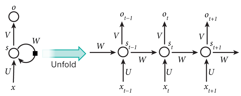
Define \(\underset{n\times m}{U}\) as the weight matrix for the input tensor, \(\underset{n\times n}{W}\) as the weight matrix for the state of the network, \(\underset{n\times 1}{b}\) as the bias vector, and \(\underset{k\times n}{V}\) as the weight matrix for the subsequent output tensor which we can ignore for now, since it technically belongs to the subsequent layer_dense.
- \(m\) is the dimension of the input tensor, i.e.
timestepsorinput_dim. - \(n\) is the dimension of the hidden layer, i.e
unitsoflayer_simple_rnn. - \(k\) is the dimension of the output tensor, i.e.
unitsof subsequentlayer_dense.
The only parameters in the model are contained within \(U\), \(W\), and \(b\), as they are shared by all steps of the RNN. Thus, the total number of parameters per layer_simple_rnn is equal to the \(dim(U)+dim(W)+dim(b)=nm+n^2+n\). In the above example, this corresponds to \(32\cdot24 + 24^2+24 = 1368\). Were we to continuing to examine the image, we would further see that:
\[ s_t = tanh(Ux_t + Ws_{t-1} + b) \\ o_t = sigmoid(Vs_t) \]
To complete this example, we see that \(s_t\) represents the output tensor of layer_simple_rnn at each timestep, and \(o_t\) the output tensor for the layer_dense. Now consider an LSTM deep learning model, which is an improvement upon the simple RNN, and equal to the previous example barring the layer type:
#LSTM example
model <- keras_model_sequential() %>%
  layer_embedding(input_dim = 1000, output_dim = 32) %>%
  layer_lstm(units = 24) %>%
  layer_dense(units = 1, activation = "sigmoid")
summary(model)
## Model: "sequential_4"
## ________________________________________________________________________________
## Layer (type) Output Shape Param #
## ================================================================================
## embedding_1 (Embedding) (None, None, 32) 32000
## ________________________________________________________________________________
## lstm (LSTM) (None, 24) 5472
## ________________________________________________________________________________
## dense_7 (Dense) (None, 1) 25
## ================================================================================
## Total params: 37,497
## Trainable params: 37,497
## Non-trainable params: 0
## ________________________________________________________________________________layer_lstm builds on layer_simple_rnn by introducing a carry dataflow to deal with the vanishing gradient problem. This results in the output tensor now being of form:
\[ s_t = tanh(Ux_t + Ws_{t-1} + c_t) \\ \]
where \(c_t\) is essentially a composite of three RNN layers, each with their own weight matrices which must be learned. Below we list the update step for the carry dataflow “parameter” \(c_t\), along with form of each piece of \(c_t\).
\[ c_{t+1} = i_t\cdot k_t + c_t \cdot f_t\\ \cdot \\ i_t = activation(U_ix_t + W_is_{t-1} + b_i)\\ f_t = activation(U_fx_t + W_fs_{t-1}+ b_f)\\ k_t = activation(U_kx_t + W_ks_{t-1} + b_k) \]
This deceptively simple refinement of layer_simple_rnn in layer_lstm also has an intuitive formula for its number of paramters. As we see, one layer_lstm is essentially like four layer_simple_rnn from a parameter point of view, and the formula for the number of parameters is correspondingly \(4(dim(U)+dim(W)+dim(b))= 4(nm+n^2+n)\). From our small example above we see that this also holds, for \(4\cdot 1368 = 5472\).
While preprocessing of images is one key subtle detail to improving the performance of a CNN, finding the correct representation (e.g. one-hot encoding, word-embeddings) is the analagous processing step needed for a succesful RNN. We only mention it here, but for more see ch. 6.1 of @dl.
In summary, RNNs work by processing sequences of inputs one timestep at a time, all while maintaining a state. Three layers are available in Keras: layer_simple_rnn, layer_lstm, and layer_gru. While recurrent layers may not be best for all problems involving sequential data, they can excel in tasks where there exist a salient, global, long-term structure in data that is predictive w.r.t. to the task at hand.
Generative deep learning
Unlike CNNs or RNNs which primarily solve well-defined spatial or temporal tasks, generative deep learning accentuates the creative potential of deep learning for more ambiguous tasks. Here we’ll briefly survey four general problems of a more creative bent: text generation, image modification through DeepDream, neural style transfer, and generative models such as VAEs or GANs. For more detail or the code, please visit: https://github.com/jjallaire/deep-learning-with-r-notebooks.
Text generation
This example explores how RNNs can be used to generate meaningful sequence data. The prevailing way to generate sequence data in deep learning is to train a network (usually an RNN or CNN) to predict the next or next few tokens using the previous tokens as input. This trained model is thought to capture the latent space of language, i.e. its statistical (and sometimes meaningful) structure. For now assume this model is a language model, given the example refers to generating text.
With a trained language model in hand, we generate new sequences by sampling from it. In more detail, we feed it an initial string of text called the conditioning data, then sample from the probability distribution for the next token. We then add this new token to the input data and repeat the process. In this example a character-level neural language model is fit, so each “probability” is the output of this LSTM model, which happens to be the softmax over all possible characters.
Generating interesting text comes down to how you sample from the probability distribution, i.e. the sampling strategy. On one end if you chose the most likely character each time the results would be incredibly repetitive with very little randomness or entropy involved. On the other, if we sampled from a uniform distribution which has the maximum amount of entropy, the results would not be meaningful at all. A happy medium would be to sample from the probability distribution as is, but there exist many potential ways of transforming the existing probability distribution to yield more interesting results.
The one implemented in this example is pretty simple. The distribution is essentially transformed and reweighted by itself, according to one user-imputed parameter called temperature, where higher temperature result in higher entropy for the new distribution, and lower temperature lower entropy. Essentially, we define a new distribution as so:
temp             <- exp(log(original_distribution) / temperature)
new_distribution <- temp / sum(temp)
Code-wise, this example is not too cumbersome to implement. The underlying model fit on the data is a recurrent DL model, specifically a single LSTM layer followed by the softmax of a dense layer for the output.
#building the model
model <- keras_model_sequential() %>%
  layer_lstm(units = 128, input_shape = c(maxlen, length(chars))) %>%
  layer_dense(units = length(chars), activation = "softmax")

optimizer <- optimizer_rmsprop(lr = 0.01)
model %>% compile(
  loss = "categorical_crossentropy",
  optimizer = optimizer
)
In addition, we define a key function sample_next_char to sample the next character given the model’s predictions. Embedded within this model is the sampling strategy we defined previously:
#reweights prob dist and samples token (char) from new dist
sample_next_char <- function(preds, temperature = 1.0) {
  preds <- as.numeric(preds)
  preds <- log(preds) / temperature
  exp_preds <- exp(preds)
  preds <- exp_preds / sum(exp_preds)
  which.max(t(rmultinom(1, 1, preds)))
}
With these two things in place all that’s left to do is to download and process the data using one-hot encoding:
#data processing for character-level text generation via LSTMs
path <- get_file(
  "nietzsche.txt",
  origin = "https://s3.amazonaws.com/text-datasets/nietzsche.txt")
text <- tolower(readChar(path, file.info(path)$size))
cat("Corpus length:", nchar(text), "\n")

#overlapping 1-hot encoded text into 3d arrays
maxlen <- 60  # Length of extracted character sequences
step <- 3  # We sample a new sequence every `step` characters

text_indexes <- seq(1, nchar(text) - maxlen, by = step)
sentences <- str_sub(text, text_indexes, text_indexes + maxlen - 1) #extr seqs
next_chars <- str_sub(text, text_indexes + maxlen, text_indexes + maxlen) #targets
cat("Number of sequences: ", length(sentences), "\n")
chars <- unique(sort(strsplit(text, "")[[1]])) #unique chars in corpus
cat("Unique characters:", length(chars), "\n")

char_indices <- 1:length(chars) #mapping unique characters to index in chars
names(char_indices) <- chars

#one-hot encode characters into binary arrays.
cat("Vectorization...\n")
x <- array(0L, dim = c(length(sentences), maxlen, length(chars)))
y <- array(0L, dim = c(length(sentences), length(chars)))
for (i in 1:length(sentences)) {
  sentence <- strsplit(sentences[[i]], "")[[1]]
  for (t in 1:length(sentence)) {
    char <- sentence[[t]]
    x[i, t, char_indices[[char]]] <- 1
  }
  next_char <- next_chars[[i]]
  y[i, char_indices[[next_char]]] <- 1
}
And using all of the tools we have defined, we finally construct the final script to generate the text. In it, we loop over epochs to fit models and generate 400 characters starting from the seed text at different temperature values.
#below trains and generates texts for a variety of temperatures
for (epoch in 1:60) {

  cat("epoch", epoch, "\n")

  # Fit the model for 1 epoch on the available training data
  model %>% fit(x, y, batch_size = 128, epochs = 1)

  # Select a text seed at random
  start_index <- sample(1:(nchar(text) - maxlen - 1), 1)
  seed_text <- str_sub(text, start_index, start_index + maxlen - 1)

  cat("--- Generating with seed:", seed_text, "\n\n")

  for (temperature in c(0.2, 0.5, 1.0, 1.2)) {

    cat("------ temperature:", temperature, "\n")
    cat(seed_text, "\n")

    generated_text <- seed_text

    # We generate 400 characters
    for (i in 1:400) {

      sampled <- array(0, dim = c(1, maxlen, length(chars)))
      generated_chars <- strsplit(generated_text, "")[[1]]
      for (t in 1:length(generated_chars)) {
        char <- generated_chars[[t]]
        sampled[1, t, char_indices[[char]]] <- 1
      }

      preds <- model %>% predict(sampled, verbose = 0)
      next_index <- sample_next_char(preds[1,], temperature)
      next_char <- chars[[next_index]]

      generated_text <- paste0(generated_text, next_char)
      generated_text <- substring(generated_text, 2)

      cat(next_char)
    }
    cat("\n\n")
  }
}
DeepDream
This example explores how representations learned by CNNs can be used to modify existing images somewhat artistically. In a nutshell, the DeepDream algorithm maximizes the activation of entire, pre-specified layers to mix together visualizations of large numbers of features, by running gradient ascent on a loss function defined by these layers at various sizes of the images, called octaves. This idea is almost identical to the CNN filter-visualization technique we discussed, where we ran the CNN in reverse, i.e. ran gradient ascent on the input to maximize the activation of a specific filter in the upper layer. The key differences are that we now maximize entire layers with a preexisting image at different octaves.
Different CNNs learn different features. Consequently, your choice of CNN for a Deep Dream naturally affects visualization. Instead of training a model from scratch, we use the InceptionV3 model, as it is is known to produce nice-looking Deep Dreams. We first load the model and disable training:
#disable any training
k_set_learning_phase(0)

#building pre-loaded incepction v3 model
model <- application_inception_v3(
  weights = "imagenet",
  include_top = FALSE
)
Now we must choose the exact set of layers whose activations we want to maximize in our loss function. Generally speaking, lower layers result in geometric patterns, while higher layers conform to the visual objects represented in the data. To better understand our choice of layers in this example, below we provide the architecture of the model.
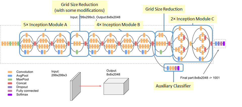
As we’ll see below, we choose the second to fifth red concatenating layer, with greater emphasis on the middle of this chain. Mixed layers are the points where the four branches of the CNN come together:
# quantifies how layer's activation contributes to the loss
layer_contributions <- list(
  mixed2 = 0.2, #names correspond to layers
  mixed3 = 3,
  mixed4 = 2,
  mixed5 = 1.5
)
Having defined which and how much each layer will contribute to the loss, we can now define the loss function. It is a weighted sum of the L2 norm of the activations of the mixed layers, which are themselves a combination of multiple activations.
# Get the symbolic outputs of each "key" layer (we gave them unique names).
layer_dict <- model$layers
names(layer_dict) <- lapply(layer_dict, function(layer) layer$name)

#defining a tensor containing our loss
loss <- k_variable(0)
for (layer_name in names(layer_contributions)) {
  coeff <- layer_contributions[[layer_name]]
  activation <- layer_dict[[layer_name]]$output #retrives layer's output
  scaling <- k_prod(k_cast(k_shape(activation), "float32"))
  loss <- loss + (coeff * k_sum(k_square(activation)) / scaling) #Add L2 norm of features of layer to loss
}
With a loss in hand, we can now define the gradient-ascent fitting algorithm to maximize the activation of the layers we chose. To do so, we leverage k_function, which properly instantiates a keras function with inputs (our generated images) and outputs (our loss function and gradients).
#setting up gradient ascent
dream <- model$input #holds current generated image, i.e. dream

#normalize gradients (imp trick)
grads <- k_gradients(loss, dream)[[1]]
grads <- grads / k_maximum(k_mean(k_abs(grads)), 1e-7)

# function to retrieve the value of loss and gradients given input image.
outputs <- list(loss, grads)
fetch_loss_and_grads <- k_function(list(dream), outputs) #inst keras func
eval_loss_and_grads <- function(x) {
  outs <- fetch_loss_and_grads(list(x))
  loss_value <- outs[[1]]
  grad_values <- outs[[2]]
  list(loss_value, grad_values)
}

#runs simple radient ascent for a number of iterations.
gradient_ascent <- function(x, iterations, step, max_loss = NULL) {
  for (i in 1:iterations) {
    c(loss_value, grad_values) %<-% eval_loss_and_grads(x)
    if (!is.null(max_loss) && loss_value > max_loss)
      break
    cat("...Loss value at", i, ":", loss_value, "\n")
    x <- x + (step * grad_values)
  }
  x
}
Finally, we can implement the Deep Dream algorithm, which requires its fair share of code. Prior to that, we define some utility functions for the algorithm. Each function resizes, saves, preprocesses, or deprocesses the image respectively:
#after upscaling we reinject details into image
resize_img <- function(img, size) {
image_array_resize(img, size[[1]], size[[2]])
}
save_img <- function(img, fname) {
img <- deprocess_image(img)
image_array_save(img, fname)
}
# Util function to open, resize, format pics into app tensors
preprocess_image <- function(image_path) {
image_load(image_path) %>%
image_to_array() %>%
array_reshape(dim = c(1, dim(.))) %>%
inception_v3_preprocess_input()
}
# Util function to converts tensor into valid image
deprocess_image <- function(img) {
img <- array_reshape(img, dim = c(dim(img)[[2]], dim(img)[[3]], 3))
img <- img / 2
img <- img + 0.5
img <- img * 255
dims <- dim(img)
img <- pmax(0, pmin(img, 255))
dim(img) <- dims
img
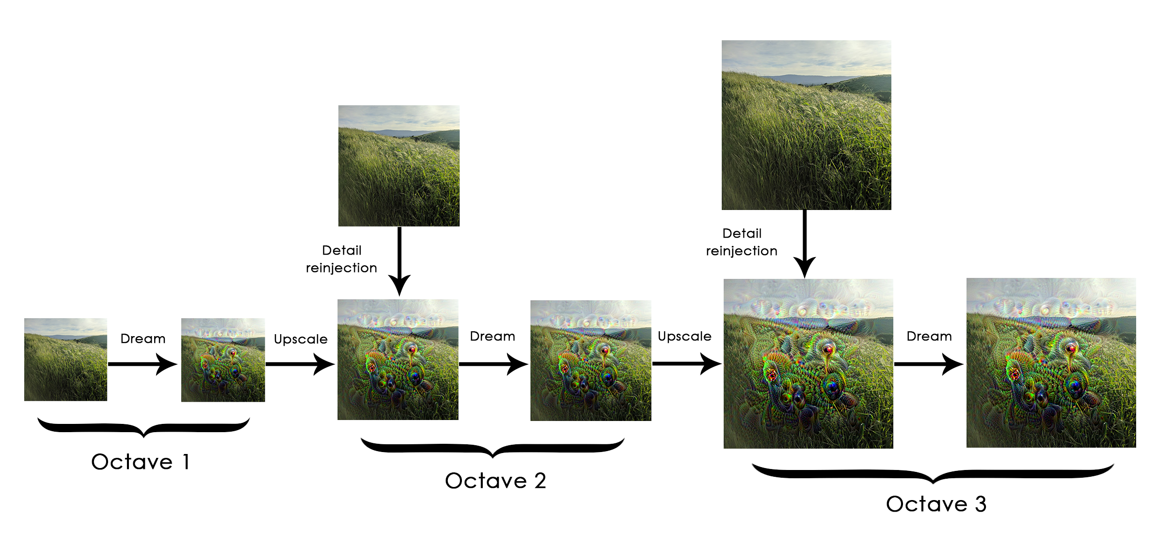
}Now the Deep Dream algorithm. Generally the idea is to process a small version of the image, run gradient ascent on the loss we defined previously to modify the image, then increase the size of the image and repeat the process. In more detail, each image is called an octave (or scale), where each successive octave is larger than the previous by a constant factor (here 1.4, i.e. 40% larger). Running gradient ascent on each octave produces the “Dream” effect. Each time we scale up, we end up losing much image detail. A fix for this is to reinject the lost details back into the image by computing the difference between the original image \(S\) and the resized image \(L\), where the difference quantifies the details lost when going from \(S\) to \(L\). This is illustrated below:
# Playing with these hyperparameters will also allow you to achieve new effects
step <- 0.01          # Gradient ascent step size
num_octave <- 3       # Number of scales at which to run gradient ascent
octave_scale <- 1.4   # Size ratio between scales
iterations <- 20      # Number of ascent steps per scale

# interrupt ga process at max_loss (10) to avoid "ugly" artifacts,
max_loss <- 10

# Fill this to the path to the image you want to use
dir.create("output/dream")
base_image_path <- "data/dream/image.jpg"
img <- preprocess_image(base_image_path) #load into array

#prepare a list of shapes for rest of code
original_shape <- dim(img)[-1]
successive_shapes <- list(original_shape)

# defining dif scales to run ga on
for (i in 1:num_octave) {
  shape <- as.integer(original_shape / (octave_scale ^ i))
  successive_shapes[[length(successive_shapes) + 1]] <- shape
}
successive_shapes <- rev(successive_shapes) #reverse list of shapes so in inc. order
original_img <- img
shrunk_original_img <- resize_img(img, successive_shapes[[1]]) #resize array of image to smallest scale

for (shape in successive_shapes) {
  cat("Processsing image shape", shape, "\n")
  img <- resize_img(img, shape)
  img <- gradient_ascent(img,
                         iterations = iterations,
                         step = step,
                         max_loss = max_loss)
  upscaled_shrunk_original_img <- resize_img(shrunk_original_img, shape)
  same_size_original <- resize_img(original_img, shape)
  lost_detail <- same_size_original - upscaled_shrunk_original_img

  img <- img + lost_detail
  shrunk_original_img <- resize_img(original_img, shape)
  save_img(img, fname = sprintf("output/dream/at_scale_%s.png",
                                paste(shape, collapse = "x")))
}

#saving and displaying results
save_img(img, fname = "output/dream/final_image_dream.png")
plot(as.raster(deprocess_image(img) / 255))
With the algorithm now in hand, here are a few examples of Deep dreams run at various configurations.
INCLUDE RESULTS HERE AFTER RUNNING ON COOL, DIFFERENT EXAMPLES.
DeepDream serves to show the versatility of applications for deep learning. Specifically, it illustrates the intriguing nature of the features the CNN learns in order to predict an outcome. Visualizing learned features is an indispensible tool in learning what exactly is going on under the hood, and DeepDream uses this to great and often trippy effect.
Neural style transfer
Neural style transfer refers to applying the visual style of a reference image to a target image, while preserving the latter’s content. While there have been many refinements of this method, we focus on the formulation found in the original paper. After mathematically defining content and style, we repeat the the same theme that is prevalent in many deep learning applications: define a loss function to specify what we want to achieve, then minimize that loss. Heuristically, we expect that loss to look something like what’s below:
#defining content/style loss (central theme in all of DL!!!) #heuristic
loss <- distance(style(reference_image) - style(generated_image)) +
  distance(content(original_image) - content(generated_image))
Here, distance is any distance metric like the \(L_2\) norm. Minimizing the obove loss function would ensure that the style of the generated_image is close to the syle of the reference_image (the one whose style we want to transfer), while preserving the content of the original_image with that of the generated_image: exactly what we want to achieve.
In this implementation we use the pre-trained VGG19 network. Roughly, the steps we must follow to generate the image with the transferred style are to:
- Set up a network that computes the VGG19 layer activations for the style-reference, target, and generated image simulateneously.
- Use these three layer activations to define the loss function.
- Set up a gradient-descent process to minimize the loss.
First we define some initial paths, dimensions for our generated image, and auxilliary functions for later.
# This is the path to the image you want to transform.
target_image_path <- "data/style/tuebingen.jpg"
# This is the path to the style image.
style_reference_image_path <- "data/style/starry_night.jpg"
# Dimensions of the generated picture.
img <- image_load(target_image_path)
width <- img$size[[1]]
height <- img$size[[2]]
img_nrows <- 400
img_ncols <- as.integer(width * img_nrows / height)

#auxilliary functions for processing the image
preprocess_image <- function(path) {
  img <- image_load(path, target_size = c(img_nrows, img_ncols)) %>%
    image_to_array() %>%
    array_reshape(c(1, dim(.)))
  imagenet_preprocess_input(img)
}
deprocess_image <- function(x) {
  x <- x[1,,,]
  # Remove zero-center by mean pixel
  x[,,1] <- x[,,1] + 103.939
  x[,,2] <- x[,,2] + 116.779
  x[,,3] <- x[,,3] + 123.68
  # 'BGR'->'RGB'
  x <- x[,,c(3,2,1)]
  x[x > 255] <- 255
  x[x < 0] <- 0
  x[] <- as.integer(x)/255
  x
}
Next we set up the VGG19 network. As input it takes a batch of three images: the style-reference image, target image, and a placeholder for the generated image. k_constant is used to define the former two since they are static, whereas k_placeholder is used to define the generated image since its dynamic, i.e. its values will change over time.
#prepping images and building VGG19 model
target_image <- k_constant(preprocess_image(target_image_path))
style_reference_image <- k_constant(
  preprocess_image(style_reference_image_path)
)
# This placeholder will contain our generated image
combination_image <- k_placeholder(c(1, img_nrows, img_ncols, 3))
input_tensor <- k_concatenate(list(target_image, style_reference_image,
                                   combination_image), axis = 1) #three images combined in a batch
# build pre-trained (ImageNet) VGG19 network with our batch of 3 images as input.
model <- application_vgg19(input_tensor = input_tensor,
                           weights = "imagenet",
                           include_top = FALSE)
Now we can define the three individual losses and the final loss comprised of the former three The content loss is defined as the \(L_2\) norm of the activations of an upper layer between the target image and the generated image. An upper layer is chosen because later layers are thought to contin more global, abstract information about the image, whereas earlier layers contain more local information. The style loss (as defined in Gatys et al.) uses the Gram matrix of multiple layers to preserve similar internal correlations within the activation of different layers across the style-reference image and the generated image. Multile layers are chosen to apture the appearance of the style-reference image at all spatial scales, and the Gram matrix b/c the inner product of the feature maps capture a map of the correlations between a layers features in a major way. A third and less-straightforward loss is the total variation loss which encourages spatial continuity in the generated image.
#Defining individual and combination losses
content_loss <- function(base, combination) {
  k_sum(k_square(combination - base))
}
gram_matrix <- function(x) {
  features <- k_batch_flatten(k_permute_dimensions(x, c(3, 1, 2)))
  gram <- k_dot(features, k_transpose(features))
  gram
}
style_loss <- function(style, combination){
  S <- gram_matrix(style)
  C <- gram_matrix(combination)
  channels <- 3
  size <- img_nrows*img_ncols
  k_sum(k_square(S - C)) / (4 * channels^2  * size^2)
}
total_variation_loss <- function(x) {
  y_ij  <- x[,1:(img_nrows - 1L), 1:(img_ncols - 1L),]
  y_i1j <- x[,2:(img_nrows), 1:(img_ncols - 1L),]
  y_ij1 <- x[,1:(img_nrows - 1L), 2:(img_ncols),]
  a <- k_square(y_ij - y_i1j)
  b <- k_square(y_ij - y_ij1)
  k_sum(k_pow(a + b, 1.25))
}
Using these three individual losses, the final loss we minimize is simply a weighted average of these three losses. For the content loss we use the block5_conv2 layer, for the style loss we use a range of layers, and the total variation loss is added at the end as it does not use any layers. One recommendation for preserving the likeness of the target image in the generated image is to increase the content_weight in the code below.
#tuning and specifiying contents, weights, etc.
# Named list mapping layer names to activation tensors
outputs_dict <- lapply(model$layers, `[[`, "output")
names(outputs_dict) <- lapply(model$layers, `[[`, "name")
# Name of layer used for content loss
content_layer <- "block5_conv2"
# Name of layers used for style loss
style_layers = c("block1_conv1", "block2_conv1",
                 "block3_conv1", "block4_conv1",
                 "block5_conv1")
# Weights in the weighted average of the loss components
total_variation_weight <- 1e-4
style_weight <- 1.0
content_weight <- 0.025
# Define the loss by adding all components to a `loss` variable
loss <- k_variable(0.0)
layer_features <- outputs_dict[[content_layer]]
target_image_features <- layer_features[1,,,]
combination_features <- layer_features[3,,,]
loss <- loss + content_weight * content_loss(target_image_features,
                                             combination_features)
for (layer_name in style_layers){
  layer_features <- outputs_dict[[layer_name]]
  style_reference_features <- layer_features[2,,,]
  combination_features <- layer_features[3,,,]
  sl <- style_loss(style_reference_features, combination_features)
  loss <- loss + ((style_weight / length(style_layers)) * sl)
}
loss <- loss +
  (total_variation_weight * total_variation_loss(combination_image))
Finally we can discuss the last piece to succesfully perform style-transfer: the gradient-descent process. Specifically, we use a custom implementation of the L-BGFS algorithm like in the original paper, except we create a custom R6 class named Evaluator to improve the efficiency of the algorithm. Whereas the algorithm originally computed the value of the loss function and the gradients independently, they are now computed jointly, where the loss is returned and the gradient is cached for the next call.
#setting up gradient descent process
# Get the gradients of the generated image wrt the loss
grads <- k_gradients(loss, combination_image)[[1]]
# Function to fetch the values of the current loss and the current gradients
fetch_loss_and_grads <- k_function(list(combination_image), list(loss, grads))
eval_loss_and_grads <- function(image) {
  image <- array_reshape(image, c(1, img_nrows, img_ncols, 3))
  outs <- fetch_loss_and_grads(list(image))
  list(
    loss_value = outs[[1]],
    grad_values = array_reshape(outs[[2]], dim = length(outs[[2]]))
  )
}
library(R6)
Evaluator <- R6Class("Evaluator",
                     public = list(

                       loss_value = NULL,
                       grad_values = NULL,

                       initialize = function() {
                         self$loss_value <- NULL
                         self$grad_values <- NULL
                       },

                       loss = function(x){
                         loss_and_grad <- eval_loss_and_grads(x)
                         self$loss_value <- loss_and_grad$loss_value
                         self$grad_values <- loss_and_grad$grad_values
                         self$loss_value
                       },

                       grads = function(x){
                         grad_values <- self$grad_values
                         self$loss_value <- NULL
                         self$grad_values <- NULL
                         grad_values
                       }
                     )
)
evaluator <- Evaluator$new()
With the setup, processing, losses, and gradient descent process finished and in play, we are now free to conduct style transfer. It works best with style-reference images that are highly textured or stylized and with easily recognizable target images. A word of warning: the algorithm is slow.
#running gradient descent process
iterations <- 20
dms <- c(1, img_nrows, img_ncols, 3)

# This is the initial state: the target image.
x <- preprocess_image(target_image_path)
# Note that optim can only process flat vectors.
x <- array_reshape(x, dim = length(x))

for (i in 1:iterations) {

  # Runs L-BFGS over the pixels of the generated image to minimize the neural style loss.
  opt <- optim(
    array_reshape(x, dim = length(x)),
    fn = evaluator$loss,
    gr = evaluator$grads,
    method = "L-BFGS-B",
    control = list(maxit = 15)
  )

  cat("Loss:", opt$value, "\n")

  image <- x <- opt$par
  image <- array_reshape(image, dms)

  im <- deprocess_image(image)
  plot(as.raster(im))
}
Analagous to the text-generation example, neural style transfer leverages the subtle, internal correlations which comprise the target image’s style together with a well-trained deep neural network to create a new work of art. While in the text-generation example we generated brand new text consistent with some style present in the seed text, here we simply transfer the existing style of a reference image onto an already existing image. Both examples serve to show the astounding versatility and reach of deep learning.
Coda
Deep learning has truly changed the game in terms of expanding the scope of tasks technology can achieve. Some believe the economic and technological impact of deep learning will be analogous to that of the internet, which may not be far from the truth given the rise of tech fueled by deep learning.
Some of its notable applications are smart assistants (Siri, Alexa, Cortana), recommender systems (Netflix, Spotify, Pandora), self-driving cars (Uber, Tesla), and emotion-recognitions systems (Affectiva). Some areas where deep learning can or has just begun to gain a footing is predictive healthcare, product quality control, doctor assistants, weather prediction, smart replies, captioning images, diet helpers, visual and video qa…the list goes on, and luckily for practitioners so does the research in this field.
While the space of possibilities for technology fueled by deep learning algorithms is vast (and still largely unconquered), it is limited. Deep learning took and extended the range of possibilities in machine learning both in terms of different data and tasks, but it is still capped by the limitations of machine learning.
Like machine learning, deep learning is still constrained to problems that can be captured algorithmically. By that, I mean problems which can be well-defined into a precise set of steps, guaranteed to terminate. This prevents any abstraction, reasoning, imagination, or improvisation, which is needed in many ambiguous and complex tasks. In addition, deep learning models are thought to generalize locally, as opposed to globally. This means that these models are great at pattern recognition and leveraging correlations in the data, but outside of a well-defined task, have trouble adapting to never-before-seen circumstances, which even a child can do. While innovations such as transfer-learning and multi-task learning are changing this second point, development of these methods is still very young.
Deep learning is just beginning to ripple through industry and changing the world as we know it in very meaningful ways. Through a zoo of methods which stack interconnected neural networks on each other, the potential for technology to improve the quality of human life is ripening. Just like fire, medicine, money, communication and transportation drastically changed the way we relate to and interact with the world and the people in it, deep learning is having a similar, albeit smaller and less noticable impact through technology. All of us are on the precipice of learning how deeply our lives may be affected by someone with a Macbook in one hand, and the world in another.
Lick the Spoon
Below we take the opportunity to review some advanced techniques useful in deep learning:
Data augmentation
Data augmentation generates additional data by applying random, label-preserving transformations to the existing data. This technique is thought to prevent overfitting and improve the generalizability of a model.
While for images the concept of a tranformation which preserves the label is straight-forward, for any data other than images it can be difficult. For example, rotating an image of a cat still means you’re looking at a cat: easy. But what would the analogy be for accelerometer data: not easy. For a good case-study on this see (Pasolli and Waldron 2017).
For images in Keras, data augmentation can convienently be done using image_data_generator.
image_data_generator - in addition to automatically converting image files on disk into batches of preprocessed tensors, this function creates new preprocessed images using existing images, i.e. data augmentation; together with flow_images_from_directory and fit_generator, these functions preprocess and feed the images into the model in batches.
For an already existing model, below are two examples of how image_data_generator fits into the model fitting pipeline. The first example will simply rescale, while the second will perform data augmentaion:
#processing data
train_datagen <- image_data_generator(rescale = 1/255)
validation_datagen <- image_data_generator(rescale = 1/255)

train_generator <- flow_images_from_directory(
  train_dir,
  train_datagen,
  target_size = c(150, 150),
  batch_size = 20,
  class_mode = "binary"
)

validation_generator <- flow_images_from_directory(
  validation_dir,
  validation_datagen,
  target_size = c(150, 150),
  batch_size = 20,
  class_mode = "binary"
)

#fitting the model - without gpu approx 15 -30 mins
history <- model %>% fit_generator(
  train_generator,
  steps_per_epoch = 100,
  epochs = 30,
  validation_data = validation_generator,
  validation_steps = 50
)
In this second example we perform data augmentation and explain some of the random transformations we perform on the image. For some code on how to view some of the images the augmentaion engine creates, please see Ch 5.2 of @dl :
#data augmentation generator
datagen <- image_data_generator(
  rescale = 1 / 255,
  rotation_range = 40,
  width_shift_range = .2,
  height_shift_range = .2,
  shear_range = .2,
  zoom_range = .2,
  horizontal_flip = T,
  fill_mode = "nearest"
)
Here’s a quick breakdown of just some of the existing options:
rotation_rangeis a value in degrees (0-180), a range within which to randomly rotate pictures.width_shiftandheight_shiftare ranges (as a fraction of total width or height) within which to randomly translate pictures vertically or horizontally.shear_rangeis for randomly applying shearing transformations.zoom_rangeis for randomly zooming inside pictures.horizontal_flipis for randomly flipping half of the images horizontally – relevant when there are no assumptions of horizontal asymmetry (e.g. real-world pictures).fill_modeis the strategy used for filling in newly created pixels, which can appear after a rotation or a width/height shift.
Having defined the generator, we can now use it in a similar manner to the first example:
#processing data with datagen (augmented data)
test_datagen <- image_data_generator(rescale = 1/255) #never augment or flow test

train_generator <- flow_images_from_directory(
  train_dir,
  datagen,   #data augmentation goes here, within
  target_size = c(150, 150),
  batch_size = 32,
  class_mode = "binary"
)
validation_generator <- flow_images_from_directory(
  validation_dir,
  test_datagen, #typo(?); for whatever reason we use test while before used validation
  target_size = c(150, 150),
  batch_size = 32,
  class_mode = "binary"
)

#fitting the model
history <- model %>% fit_generator(
  train_generator,
  steps_per_epoch = 100,
  epochs = 100,
  validation_data = validation_generator,
  validation_steps = 50
)
Regularization
This is a technique to mitigate overfitting by puttings constraints on the model such that parameters are forced to take small values, i.e it makes the distribution of parameters more regular. This is done by taking the existing loss function for a model, and adding a penalty or cost to it for having large parameter values. These ideas for penalizing the loss function originated under the name of Lasso and Ridge regression, and their primary motivation was to deal with correlated predictors.
In Keras the choice of penalty is either \(L_1\), \(L_2\), or a mix of both. This is by inserting one of three functions into the kernal_regularizer option available in any layer:
regularizer_l1() - implements \(L_1\) penalty on loss.
regularizer_l2() - implements \(L_2\) penalty on loss.
regularizer_l1_l2() - implements both \(L_1\) and \(L_2\) penalty on loss.
Below is an example of a model which utilizes regularization in both layers:
l2_model <- keras_model_sequential() %>%
  layer_dense(units = 16, kernel_regularizer = regularizer_l2(0.001),
              activation = "relu", input_shape = c(10000)) %>%
  layer_dense(units = 16, kernel_regularizer = regularizer_l2(0.001),
              activation = "relu") %>%
  layer_dense(units = 1, activation = "sigmoid")
l2_model %>% compile(
  optimizer = "rmsprop",
  loss = "binary_crossentropy",
  metrics = c("acc")
)
regularizer_l2(0.001) means every coefficient in the weight matrix of the layer will add 0.001 * weight_coefficient_value to the total loss of the network. Note that because this penalty is only added at training time, the loss for this network will be much higher at training than at test time.
Dropout
This is another regularization technique which prevents overfitting by randomly dropping out (i.e. setting to zero) a number of output features for some layer during training. For example if a layer was set to return 0.2, 0.5, 1.3, 0.8, 1.1, after applying a dropout layer it may return 0, 0.5, 0, 0.8, 1.1, depending on the dropout rate.
The dropout rate refers to the fraction of features that are zeroed out; typical numbers range from 0.2 to 0.5. These layers are prevalent in many of the larger, successful models such as VGG, ResNet, Inception and so on. While we drop out layers during training, at test time instead scale down that layer’s output values by a factor equal to the dropout rate, as an adjustment for there being more active units at training time. In practice, both of these operations are done during training (we scale the output layer in training up instead of down), leaving testing unchanged. In other words at training time:
# At training time:
layer_output <- layer_output * sample(0:1, length(layer_output), replace = TRUE)
layer_output <- layer_output / 0.5 #note the scaling up
In keras, we implement the above pseudocode through layer_dropout():
layer_dropout() - randomly sets a fraction rate of inputs to 0 at each update during training, primarily through rate.
Here we improve the results of the previous IMDB model using layer_dropout.
dpt_model <- keras_model_sequential() %>%
  layer_dense(units = 16, activation = "relu", input_shape = c(10000)) %>%
  layer_dropout(rate = 0.5) %>%
  layer_dense(units = 16, activation = "relu") %>%
  layer_dropout(rate = 0.5) %>%
  layer_dense(units = 1, activation = "sigmoid")
dpt_model %>% compile(
  optimizer = "rmsprop",
  loss = "binary_crossentropy",
  metrics = c("acc")
)
Batch normalization
Normalization refers to a group of methods for making observations more similar to each other while retaining certain unique aspects of the data, such as variability. Its key utility is that it helps propogate the gradient throughout training; in fact, most large deep learning models packaged in keras (such as ResNet50, Inception V3, and Xception) wont converge without it. One of the most common ways to normalize the data is to subtract the mean from all observations and divide each one by its standard deviation (assumes data is normally distributed), resulting in centered data with scaled variability.
Normalizing data before feeding it into a model is to be expected, but in deep learning the data may no longer be normalized when feeding into subsequent layers, creating a need for additional normalization between layers. Most advanced CNNs use layer_batch_normalization liberally in their models, and typically after a convolutional or densely connected layer.
layer_batch_normalization() - adaptively normalizes even as mean and variance change during training; done by retaining an exponential moving average of the batch-wise mean and variance; takes an axis argument to specify feature axis for normalization, where the default is -1 for the last axis in the input tensor, which is correct for many layer types since they use the channels last convention.
layer_conv_2d(filters = 32, kernel_size = 3, activation = "relu") %>%
  layer_batch_normalization()

layer_dense(units = 32, activation = "relu") %>%
  layer_batch_normalization()
In the future, batch renormalization (introduced by Ioffe in 2017) may replace batch normalization, but for now the layer_batch_normalization is still an effective tool to propogate the gradient during training.
Pretrained DL models
A useful pretrained network refers to a saved network that was previously trained on a dataset that was preferably large. A large, general previous dataset is preferred because it suggests that the spatial hierachy of features learned by the model is general enough to still prove useful on tasks much different than the original. There exist two ways to leverage a pretrained network for a new task: feature extraction and fine-tuning. We’ll cover both within the context of CNNs.
Feature Extraction
Feature extraction uses the existing model to extract interesting new features from new samples, then runs these features through a new classifier that is trained from scratch. As mentioned earlier, earlier layers in the model are thought to capture the more generic features such as visual edges, colors, and textures, while later layers are though to capture more abstract concepts of the data such as “cat ear” or “dog eye”. For this reason, unless the new task is very similar to the old one. it is recommneded to use the earlier part of the convolutional base when extracting useful features.
To begin, the first step is to instantiate an existing model, of which there are many which come prepackaged in keras, some of the most popular being Xception, Inception V3, ResNet50, VGG 16, VGG 19, MobileNet. We choose VGG16:
conv_base <- application_vgg16(
  weights = "imagenet",
  include_top = FALSE,
  input_shape = c(150, 150, 3)
)
In all of the pre-loaded models, there are three arguments to pass in:
weights - specifies the weights from which to initialize the model.
include_top - denotes whether you want to include the densely connected classifier layer at the end of the model; almost always this is FALSE to use it on a new task.
input_shape - optional argument to specify the shape of the tensors we feed into the model.
With these already in place above, we can print out a summary of this CNN base we’ll use to extract features:
conv_base## Model
## Model: "vgg16"
## ________________________________________________________________________________
## Layer (type) Output Shape Param #
## ================================================================================
## input_1 (InputLayer) [(None, 150, 150, 3)] 0
## ________________________________________________________________________________
## block1_conv1 (Conv2D) (None, 150, 150, 64) 1792
## ________________________________________________________________________________
## block1_conv2 (Conv2D) (None, 150, 150, 64) 36928
## ________________________________________________________________________________
## block1_pool (MaxPooling2D) (None, 75, 75, 64) 0
## ________________________________________________________________________________
## block2_conv1 (Conv2D) (None, 75, 75, 128) 73856
## ________________________________________________________________________________
## block2_conv2 (Conv2D) (None, 75, 75, 128) 147584
## ________________________________________________________________________________
## block2_pool (MaxPooling2D) (None, 37, 37, 128) 0
## ________________________________________________________________________________
## block3_conv1 (Conv2D) (None, 37, 37, 256) 295168
## ________________________________________________________________________________
## block3_conv2 (Conv2D) (None, 37, 37, 256) 590080
## ________________________________________________________________________________
## block3_conv3 (Conv2D) (None, 37, 37, 256) 590080
## ________________________________________________________________________________
## block3_pool (MaxPooling2D) (None, 18, 18, 256) 0
## ________________________________________________________________________________
## block4_conv1 (Conv2D) (None, 18, 18, 512) 1180160
## ________________________________________________________________________________
## block4_conv2 (Conv2D) (None, 18, 18, 512) 2359808
## ________________________________________________________________________________
## block4_conv3 (Conv2D) (None, 18, 18, 512) 2359808
## ________________________________________________________________________________
## block4_pool (MaxPooling2D) (None, 9, 9, 512) 0
## ________________________________________________________________________________
## block5_conv1 (Conv2D) (None, 9, 9, 512) 2359808
## ________________________________________________________________________________
## block5_conv2 (Conv2D) (None, 9, 9, 512) 2359808
## ________________________________________________________________________________
## block5_conv3 (Conv2D) (None, 9, 9, 512) 2359808
## ________________________________________________________________________________
## block5_pool (MaxPooling2D) (None, 4, 4, 512) 0
## ================================================================================
## Total params: 14,714,688
## Trainable params: 14,714,688
## Non-trainable params: 0
## ________________________________________________________________________________The final layer on which we add our densely connected classifier has shape (4, 4, 512). At this point there are two approaches: a fast and slow one. The fast approach runs the conv_base over the new dataset, records the output, then uses this output as input data in a standalone and simple DL model such as this:
model <- keras_model_sequential() %>%
  layer_dense(units = 256, activation = "relu",
              input_shape = 4 * 4 * 512) %>%
  layer_dropout(rate = 0.5) %>%
  layer_dense(units = 1, activation = "sigmoid")

model
## Model
## Model: "sequential_5"
## ________________________________________________________________________________
## Layer (type) Output Shape Param #
## ================================================================================
## dense_8 (Dense) (None, 256) 2097408
## ________________________________________________________________________________
## dropout (Dropout) (None, 256) 0
## ________________________________________________________________________________
## dense_9 (Dense) (None, 1) 257
## ================================================================================
## Total params: 2,097,665
## Trainable params: 2,097,665
## Non-trainable params: 0
## ________________________________________________________________________________This approach is fast because there is only a small amount of training required for the simple model. There is more upfront work though to extract and reshape the features appropriately. One drawback is that you cannot perform data augmentation, which is a critical tool with small datasets.
The slow approach is to extend conv_base by adding the simple model (which includes the densely connected classfier) onto it, and running this combined model end to end on the input data. This allows us to use data augmentation, but for that reason is much slower, and even intractable without a GPU setup. Here is an example of adding to conv_base in the slow approach:
model <- keras_model_sequential() %>%
  conv_base %>%
  layer_flatten() %>%
  layer_dense(units = 256, activation = "relu") %>%
  layer_dense(units = 1, activation = "sigmoid")

model
## Model
## Model: "sequential_6"
## ________________________________________________________________________________
## Layer (type) Output Shape Param #
## ================================================================================
## vgg16 (Model) (None, 4, 4, 512) 14714688
## ________________________________________________________________________________
## flatten_2 (Flatten) (None, 8192) 0
## ________________________________________________________________________________
## dense_10 (Dense) (None, 256) 2097408
## ________________________________________________________________________________
## dense_11 (Dense) (None, 1) 257
## ================================================================================
## Total params: 16,812,353
## Trainable params: 16,812,353
## Non-trainable params: 0
## ________________________________________________________________________________When fitting this model, a crucial note is that the models in the base must be frozen so that the previously learned representations are not destroyed. This is done easily through freeze_weights. Note the number of learnable parameters before (see above print out of model) and after (below model printout) freezing the weights in conv_base:
freeze_weights(conv_base)
model
## Model
## Model: "sequential_6"
## ________________________________________________________________________________
## Layer (type) Output Shape Param #
## ================================================================================
## vgg16 (Model) (None, 4, 4, 512) 14714688
## ________________________________________________________________________________
## flatten_2 (Flatten) (None, 8192) 0
## ________________________________________________________________________________
## dense_10 (Dense) (None, 256) 2097408
## ________________________________________________________________________________
## dense_11 (Dense) (None, 1) 257
## ================================================================================
## Total params: 16,812,353
## Trainable params: 2,097,665
## Non-trainable params: 14,714,688
## ________________________________________________________________________________For the further details and implementations of both of these methods, please refer to the source text. Interestingly enough, both of these approaches yield validation accuracies of roughly 90%, but the former trains much faster than the latter. And while this next method is also time-consuming, we’ll see a much higher accuracy of 96&.
Fine-Tuning
Fine-tuning is similar to the slow method we just described, in that we unfreeze a few of the later layers and retrain the model end to end again. Fine-tuning refers to the fact that these abstract, later representations are being retrained or tuned to make them more relevant to the new task. The key difference is the procedure we must follow to avoid destroying the previously learned representations in conv_base. Here are the steps for fine-tuning a model:
- Add custom network on top of an already-trained base network.
- Freeze the base network.
- Train the part you just added.
- Unfreeze some of the layers in the base network.
- Jointly train both of these layers and the part we just added.
If you haven’t already noticed, steps 1-3 precisely describe the slow method. So really, step 4 and 5 are the only additional steps needed to fine-tune the model. We’ll continue the steps we initiated above in the example. Below we print out the frozen conv_base, to illustrate how we’ll use layers from block3_conv1 onwards to fine-tune the model:
conv_base## Model
## Model: "vgg16"
## ________________________________________________________________________________
## Layer (type) Output Shape Param #
## ================================================================================
## input_1 (InputLayer) [(None, 150, 150, 3)] 0
## ________________________________________________________________________________
## block1_conv1 (Conv2D) (None, 150, 150, 64) 1792
## ________________________________________________________________________________
## block1_conv2 (Conv2D) (None, 150, 150, 64) 36928
## ________________________________________________________________________________
## block1_pool (MaxPooling2D) (None, 75, 75, 64) 0
## ________________________________________________________________________________
## block2_conv1 (Conv2D) (None, 75, 75, 128) 73856
## ________________________________________________________________________________
## block2_conv2 (Conv2D) (None, 75, 75, 128) 147584
## ________________________________________________________________________________
## block2_pool (MaxPooling2D) (None, 37, 37, 128) 0
## ________________________________________________________________________________
## block3_conv1 (Conv2D) (None, 37, 37, 256) 295168
## ________________________________________________________________________________
## block3_conv2 (Conv2D) (None, 37, 37, 256) 590080
## ________________________________________________________________________________
## block3_conv3 (Conv2D) (None, 37, 37, 256) 590080
## ________________________________________________________________________________
## block3_pool (MaxPooling2D) (None, 18, 18, 256) 0
## ________________________________________________________________________________
## block4_conv1 (Conv2D) (None, 18, 18, 512) 1180160
## ________________________________________________________________________________
## block4_conv2 (Conv2D) (None, 18, 18, 512) 2359808
## ________________________________________________________________________________
## block4_conv3 (Conv2D) (None, 18, 18, 512) 2359808
## ________________________________________________________________________________
## block4_pool (MaxPooling2D) (None, 9, 9, 512) 0
## ________________________________________________________________________________
## block5_conv1 (Conv2D) (None, 9, 9, 512) 2359808
## ________________________________________________________________________________
## block5_conv2 (Conv2D) (None, 9, 9, 512) 2359808
## ________________________________________________________________________________
## block5_conv3 (Conv2D) (None, 9, 9, 512) 2359808
## ________________________________________________________________________________
## block5_pool (MaxPooling2D) (None, 4, 4, 512) 0
## ================================================================================
## Total params: 14,714,688
## Trainable params: 0
## Non-trainable params: 14,714,688
## ________________________________________________________________________________Unfreezing the weights so we can jointly train our addition to the model with the unfrozen layers is done using the unfreeze_weights function:
unfreeze_weights(conv_base, from = "block5_conv1")
conv_base
## Model
## Model: "vgg16"
## ________________________________________________________________________________
## Layer (type) Output Shape Param #
## ================================================================================
## input_1 (InputLayer) [(None, 150, 150, 3)] 0
## ________________________________________________________________________________
## block1_conv1 (Conv2D) (None, 150, 150, 64) 1792
## ________________________________________________________________________________
## block1_conv2 (Conv2D) (None, 150, 150, 64) 36928
## ________________________________________________________________________________
## block1_pool (MaxPooling2D) (None, 75, 75, 64) 0
## ________________________________________________________________________________
## block2_conv1 (Conv2D) (None, 75, 75, 128) 73856
## ________________________________________________________________________________
## block2_conv2 (Conv2D) (None, 75, 75, 128) 147584
## ________________________________________________________________________________
## block2_pool (MaxPooling2D) (None, 37, 37, 128) 0
## ________________________________________________________________________________
## block3_conv1 (Conv2D) (None, 37, 37, 256) 295168
## ________________________________________________________________________________
## block3_conv2 (Conv2D) (None, 37, 37, 256) 590080
## ________________________________________________________________________________
## block3_conv3 (Conv2D) (None, 37, 37, 256) 590080
## ________________________________________________________________________________
## block3_pool (MaxPooling2D) (None, 18, 18, 256) 0
## ________________________________________________________________________________
## block4_conv1 (Conv2D) (None, 18, 18, 512) 1180160
## ________________________________________________________________________________
## block4_conv2 (Conv2D) (None, 18, 18, 512) 2359808
## ________________________________________________________________________________
## block4_conv3 (Conv2D) (None, 18, 18, 512) 2359808
## ________________________________________________________________________________
## block4_pool (MaxPooling2D) (None, 9, 9, 512) 0
## ________________________________________________________________________________
## block5_conv1 (Conv2D) (None, 9, 9, 512) 2359808
## ________________________________________________________________________________
## block5_conv2 (Conv2D) (None, 9, 9, 512) 2359808
## ________________________________________________________________________________
## block5_conv3 (Conv2D) (None, 9, 9, 512) 2359808
## ________________________________________________________________________________
## block5_pool (MaxPooling2D) (None, 4, 4, 512) 0
## ================================================================================
## Total params: 14,714,688
## Trainable params: 7,079,424
## Non-trainable params: 7,635,264
## ________________________________________________________________________________To better illustrate how we have fine-tuned the original VGG16 model, consider the image below, where blue represents frozen layers, and green the layers we intent to train.
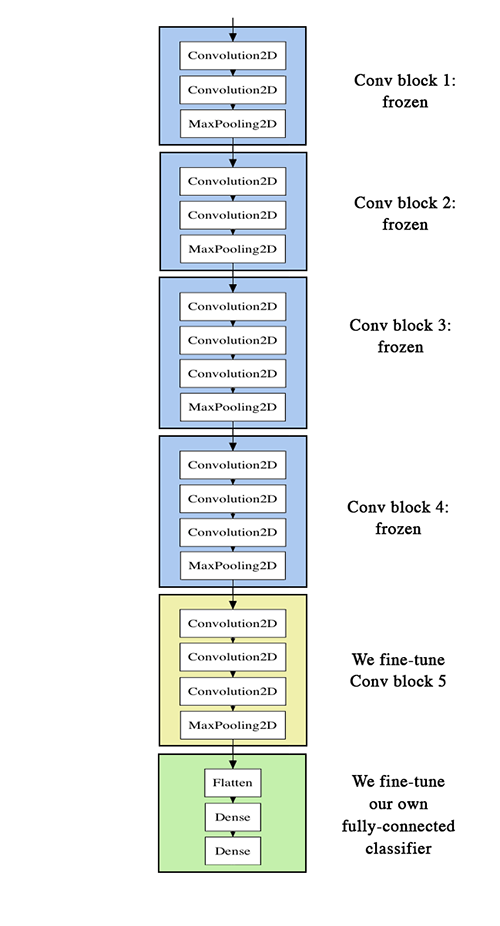
To actually achieve the high performance of 96% accuracy, we must unfreeze most of the VGG16 model, specifically from block3_conv1 onwards. We do that below and include the code necessary to fit the final model. One key detail is taht we use the RMSProp optimizer with a very slow learning rate in an attempt to limit the mangnitude of modifications to the three-layers we’re fine-tuning:
unfreeze_weights(conv_base, from = "block3_conv1")
conv_base

model %>% compile(
  loss = "binary_crossentropy",
  optimizer = optimizer_rmsprop(lr = 1e-5),
  metrics = c("accuracy")
)
history <- model %>% fit_generator(
  train_generator,
  steps_per_epoch = 100,
  epochs = 100,
  validation_data = validation_generator,
  validation_steps = 50
)
Feature extraction through any of these three methods would be useful in improving the performance of a deep learning model, especially in the case where data is not very large. Often it is costly to obtain, manage, and process such data, so these methods are incredibly relevant for building high-performing models.
Pretrained features in RNNs
In RNNs we can use this idea of feature extraction as well. Take for example the movie sentiment task where the data consists of movie reviews. Instead of trying to learn from scratch features or embeddings jointly with building a good classifier, we can use pretrained word embeddings. The motivation for doing this is the same as the previous example: we don’t have enough data to learn truly powerful features. Just as in CNNs, there exists various precomputed databases built into keras, such as word2vec and glove. The code to use pretrained embeddings is slightly more hands-on, so we’ll leave the demonstration to the book.
The notion that we can re-use existing models in this way is very appealing, and speaks to the versatility of deep learning. It is an option in both CNNs and RNNs, and is most useful when we lack the the resources (time, data, computational power) to learn truly powerful features on our own.
Visualizing CNNs for interpretation
Ordinarily, interpreting a deep learning model is near-impossible due to the utter complexity in even the simplest models, but this is not exactly the case with CNNs. In CNNs the feature maps are thought to capture representations of visual concepts, making them amenable to visualization and therefore interpretation. In this small section we’ll survey three of the most important methods for visualizing a model:
- Visualizing intermediate CNN outputs (i.e. intermediate activations) - helps understand how successive layers are transforming an input, and gives intuition about the meaning behind individual filters.
- Visualizing CNN filters - helps understand what visual pattern or concept a particular filter is maximally receptive to; displays the “basis images” which decompose a particular input to predict a task.
- Visualizing heatmaps of class activation in an image - helps identify which parts of an image are identified as belonging to a given class; answers why a certain image is predicted to belong to a certain class by highlighting an area of the image.
Intermediate CNN outputs
Visualizing intermediate activations consists of displaying the outputted feature maps or activations of various convolutional or pooling layers for a given input image. These activations give a glimpse into how the input is decomposed by different layers. Each feature map has 3 dimensions we must visualize (width, height, depth i.e channels), and each channel encodes relatively independent features surprisingly enough. Consequently, it is advicsed to visualize the feature maps by plotting the contents of every channel. We first load the model and preprocess and display an image we’ll use to illustrate this technique.
#loading and viewing model
model <- load_model_hdf5("files/cats_and_dogs_small_2.h5")
summary(model)
## Model: "sequential_1"
## ________________________________________________________________________________
## Layer (type) Output Shape Param #
## ================================================================================
## conv2d_4 (Conv2D) (None, 148, 148, 32) 896
## ________________________________________________________________________________
## max_pooling2d_4 (MaxPooling2D) (None, 74, 74, 32) 0
## ________________________________________________________________________________
## conv2d_5 (Conv2D) (None, 72, 72, 64) 18496
## ________________________________________________________________________________
## max_pooling2d_5 (MaxPooling2D) (None, 36, 36, 64) 0
## ________________________________________________________________________________
## conv2d_6 (Conv2D) (None, 34, 34, 128) 73856
## ________________________________________________________________________________
## max_pooling2d_6 (MaxPooling2D) (None, 17, 17, 128) 0
## ________________________________________________________________________________
## conv2d_7 (Conv2D) (None, 15, 15, 128) 147584
## ________________________________________________________________________________
## max_pooling2d_7 (MaxPooling2D) (None, 7, 7, 128) 0
## ________________________________________________________________________________
## flatten_1 (Flatten) (None, 6272) 0
## ________________________________________________________________________________
## dropout (Dropout) (None, 6272) 0
## ________________________________________________________________________________
## dense_2 (Dense) (None, 512) 3211776
## ________________________________________________________________________________
## dense_3 (Dense) (None, 1) 513
## ================================================================================
## Total params: 3,453,121
## Trainable params: 3,453,121
## Non-trainable params: 0
## ________________________________________________________________________________#preprocessing image into 4d tensor
img_path <- "files/cat.1700.jpg"
img <- image_load(img_path, target_size = c(150, 150))
img_tensor <- image_to_array(img)
img_tensor <- array_reshape(img_tensor, c(1, 150, 150, 3))
img_tensor <- img_tensor / 255 #images were preprocessed this way
dim(img_tensor)## [1] 1 150 150 3plot(as.raster(img_tensor[1,,,]))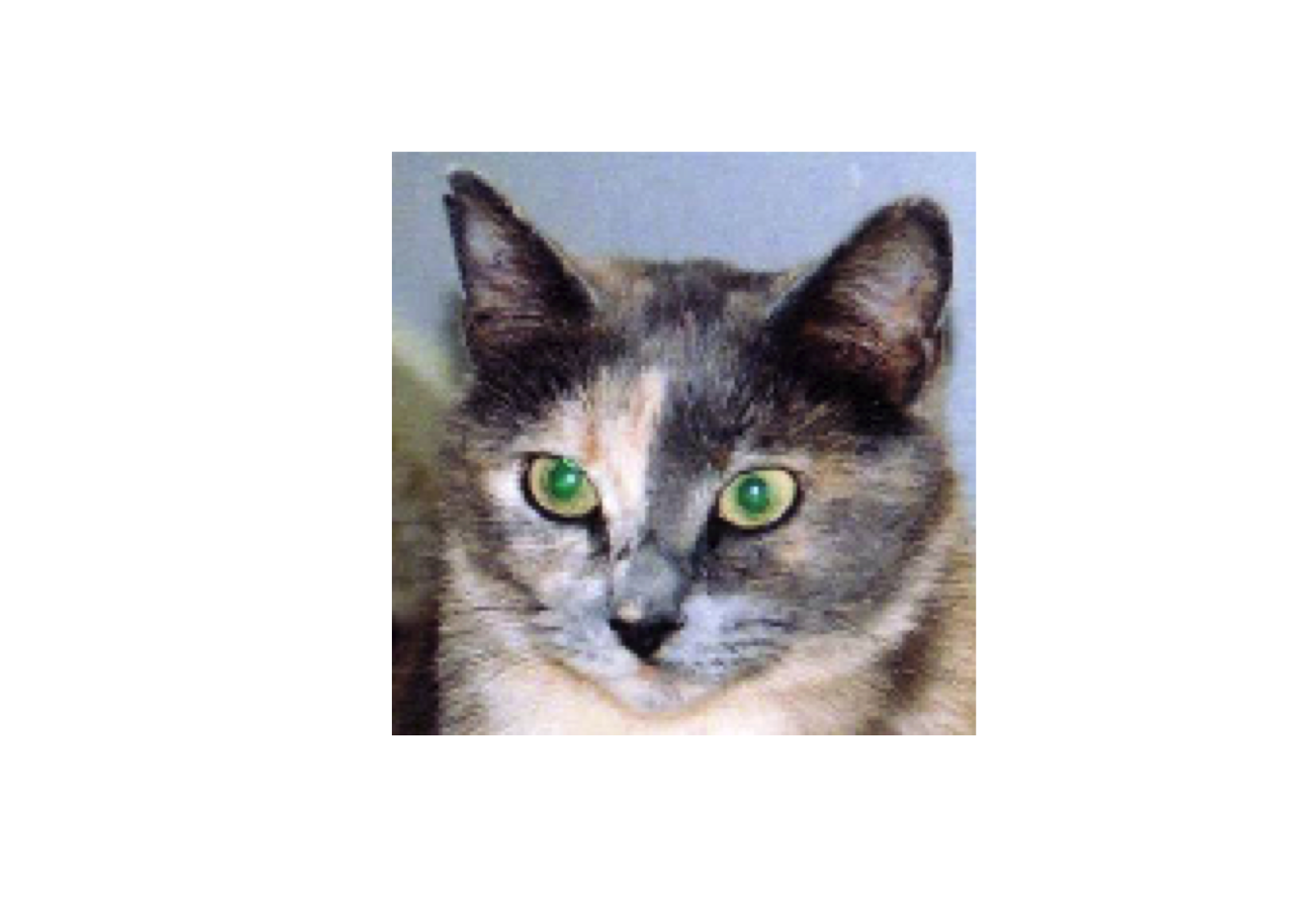
With the input image in place, we can now begin plotting some sample images run through the feature maps. To extract the feature maps of interest, we must create a Keras model that takes batches of images as input, and reutrns activations of all convolutional and pooling layers. To do this we use keras_model which takes and input tensor (or list of input tensors) along with an output tensor (or list of output tensors) and can return multiple outputs, unlike keras_model_sequential:
#extracts output from top 8 layers:
layer_outputs <- lapply(model$layers[1:8], function(layer) layer$output)
activation_model <- keras_model(inputs = model$input, outputs = layer_outputs) #returns outputs given inputs
# Returns a list of five arrays: one array per layer activation
activations <- activation_model %>% predict(img_tensor)
first_layer_activation <- activations[[1]]
dim(first_layer_activation) #one 148x148 feature map with 32 channels

#defining and applying function to plot a channel
plot_channel <- function(channel) {
  rotate <- function(x) t(apply(x, 2, rev))
  image(rotate(channel), axes = FALSE, asp = 1,
        col = terrain.colors(12))
}

plot_channel(first_layer_activation[1,,,6]) #edge detector
plot_channel(first_layer_activation[1,,,1]) #eyes + nose
plot_channel(first_layer_activation[1,,,9]) #ears, eyes + nose
In these channels (6th, 1st, and 9th) of the first layer, there seems to be some edge detection occurring with a recurring focus on the eyes and nose of the cat. To visualize all of the activations in the network, we can plot every channel in each of our 8 activation maps, with results in one big input tensor where the channels are stacked side by side.
dir.create("output/cat_activations")
image_size <- 58
images_per_row <- 16
for (i in 1:8) {

  layer_activation <- activations[[i]]
  layer_name <- model$layers[[i]]$name

  n_features <- dim(layer_activation)[[4]]
  n_cols <- n_features %/% images_per_row

  png(paste0("output/cat_activations/", i, "_", layer_name, ".png"),
      width = image_size * images_per_row,
      height = image_size * n_cols)
  op <- par(mfrow = c(n_cols, images_per_row), mai = rep_len(0.02, 4))

  for (col in 0:(n_cols-1)) {
    for (row in 0:(images_per_row-1)) {
      channel_image <- layer_activation[1,,,(col*images_per_row) + row + 1]
      plot_channel(channel_image)
    }
  }

  par(op)
  dev.off()
}
Now we finally the heuristic we’ve mentioned where deep learning models tent to encode more general features in earlier layers, where later layers encode more abstract features such as ear or eye. Although the actual tranformations occuring to the image are hard to interpret with respect to the task, this techniqe is very powerful when combined the two following ones.
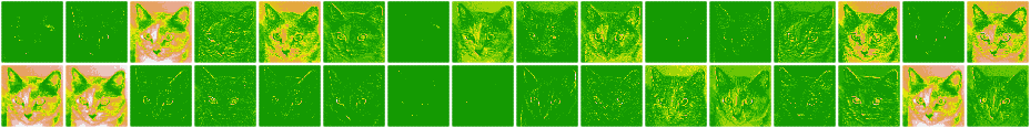
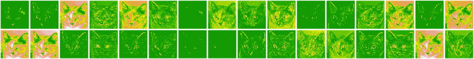
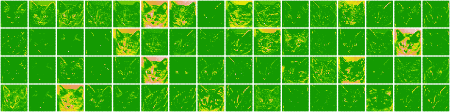
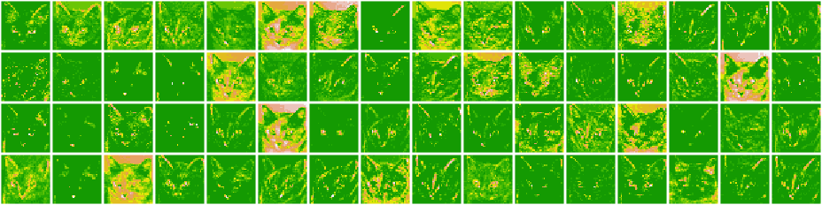
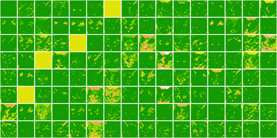
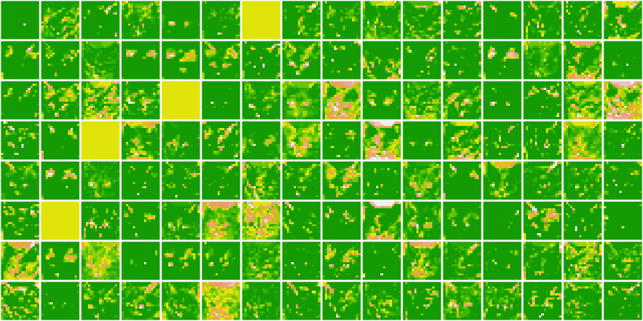
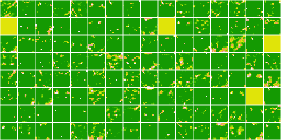
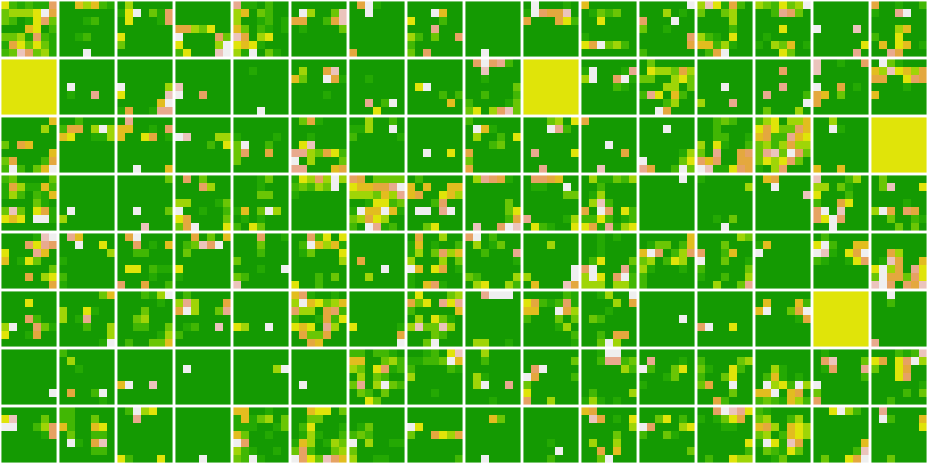
CNN filters
Visualizing the pattern that a filter is thought to maximally respond to is a useful approach to try and interpret the behavior of a model. This is done by applying gradient descent the value of a blank input image to maximize the response of a specific filter. So in essence, we apply gradient ascent in the input space.
To code this we must define a loss function which maximizes the value of a given CNN filter, then use SGD to adjust the values of the input image to maximize the activation value. In the following example we start by defining a loss for the activation of filter 1 in layer block3_conv1 of the pretrained VGG16 network from ImageNet. Note: some backend functions for keras were used, such as k_mean_, k_gradients, and iterate:
model <- application_vgg16(
  weights = "imagenet",
  include_top = FALSE
)

layer_name   <- "block3_conv1"
filter_index <- 1
layer_output <- get_layer(model, layer_name)$output
loss <- k_mean(layer_output[,,,filter_index])

#need gradient of loss wrt to model input; keep only 1 element of list of tensors
grads <- k_gradients(loss, model$input)[[1]]
grads <- grads / (k_sqrt(k_mean(k_square(grads))) + 1e-5) #avoids dividing by 0
iterate <- k_function(list(model$input), list(loss, grads))

#testing iterate to compute loss and gradient
c(loss_value, grads_value) %<-%
    iterate(list(array(0, dim = c(1, 150, 150, 3))))

#loop to perform sgd, starting from a gray image with some noise
input_img_data <-
  array(runif(150 * 150 * 3), dim = c(1, 150, 150, 3)) * 20 + 128
step <- 1  #magnitude of each gradient update
for (i in 1:40) {
  c(loss_value, grads_value) %<-% iterate(list(input_img_data)) #compute loss + gradient
  input_img_data <- input_img_data + (grads_value * step) #adjust input to max loss
}
One trick we use above is to normalize the gradient tensor by dividing by its \(L_2\) norm to ensure the magnitude of the updates on the input image is always within the same range. The resulting image tensor is a floating-point tensor of shape (1, 150, 150, 3), with values potentially outside [0, 255]. To make the image “displayable”, we postprocess the image with deprocess_image.
deprocess_image normalizes, bounds, and returns a tensor of identical input shape. In addition, we define the key_function generate_pattern which takes a layer name and filter index to return a valid image tensor with the pattern which maximixes the activation of that specific filter.
deprocess_image <- function(x) {

  dms <- dim(x)
  # normalize tensor: center on 0., ensure std is 0.1
  x <- x - mean(x)
  x <- x / (sd(x) + 1e-5)
  x <- x * 0.1

  # clip to [0, 1]
  x <- x + 0.5
  x <- pmax(0, pmin(x, 1))

  # Reshape to original image dimensions
  array(x, dim = dms)
}

generate_pattern <- function(layer_name, filter_index, size = 150) {

  #Build a loss function that maximizes the activation
  # of the nth filter of the layer considered.
  layer_output <- model$get_layer(layer_name)$output
  loss <- k_mean(layer_output[,,,filter_index])

  #Compute the gradient of the input picture wrt this loss
  grads <- k_gradients(loss, model$input)[[1]]

  #Normalization trick: we normalize the gradient
  grads <- grads / (k_sqrt(k_mean(k_square(grads))) + 1e-5)

  # his function returns the loss and grads given the input picture
  iterate <- k_function(list(model$input), list(loss, grads))

  #We start from a gray image with some noise
  input_img_data <-
    array(runif(size * size * 3), dim = c(1, size, size, 3)) * 20 + 128

  #Run gradient ascent for 40 steps
  step <- 1
  for (i in 1:40) {
    c(loss_value, grads_value) %<-% iterate(list(input_img_data))
    input_img_data <- input_img_data + (grads_value * step)
  }
  img <- input_img_data[1,,,]
  deprocess_image(img)
}

#plotting the first filter of the layer below
library(grid)
grid.raster(generate_pattern("block3_conv1", 1))
If you ran this code you would see a polk-dot pattern, indicating that that filter is maximally response to a polka-dot pattern.
With all the pieces in place, we can know visualize every filter in every layer if we wished. For ease, we reproduce the first layer of each convolutional layer in this model.
library(grid)
library(gridExtra)
dir.create("images/vgg_filters")
for (layer_name in c("block1_conv1", "block2_conv1",
                     "block3_conv1", "block4_conv1",
                     "block5_conv1")) {
  size <- 140

  png(paste0("images/vgg_filters/", layer_name, ".png"),
      width = 8 * size, height = 8 * size)

  grobs <- list()
  for (i in 0:7) {
    for (j in 0:7) {
      pattern <- generate_pattern(layer_name, i + (j*8) + 1, size = size)
      grob <- rasterGrob(pattern,
                         width = unit(0.9, "npc"),
                         height = unit(0.9, "npc"))
      grobs[[length(grobs)+1]] <- grob
    }
  }

  grid.arrange(grobs = grobs, ncol = 8)
  dev.off()
}
Much like a Fourier basis decomposition find a represention for each function in FDA using combinations of sine and consine functions, each layer in a CNN learns a collection of filters such that their inputs can be expressed as a combination of those filters. We finally see the pattern that we had alluded to throughout the document, where earlier layers are very general and later laters tend to code more abstract features specific to the data such as eyes:
block1_conv1
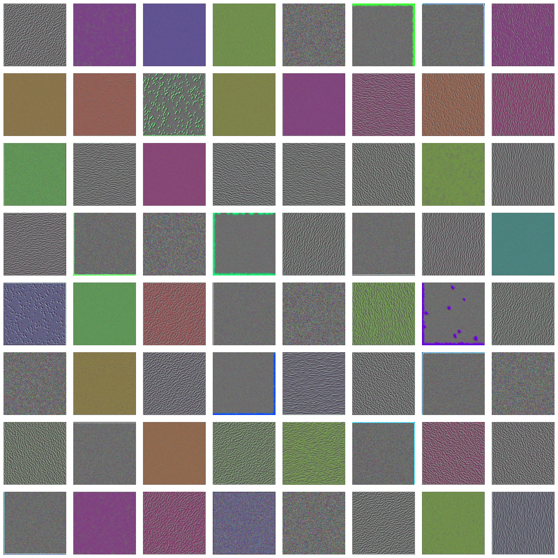
block2_conv1
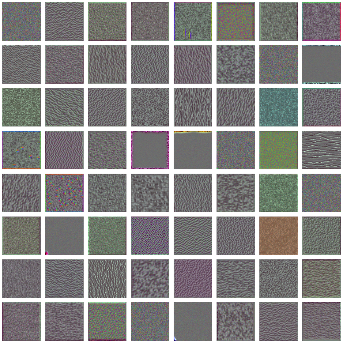
block3_conv1
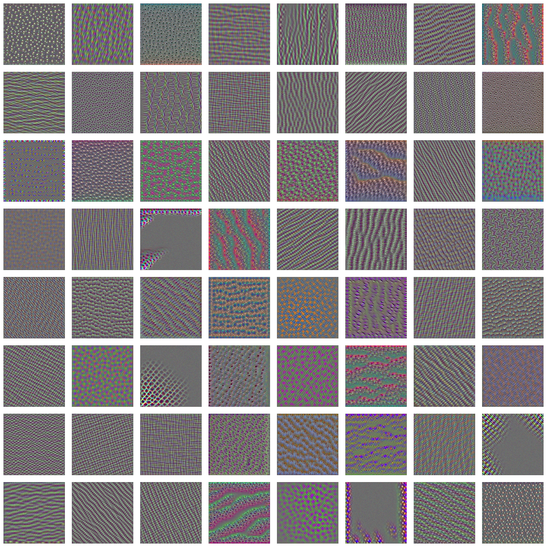
block4_conv1
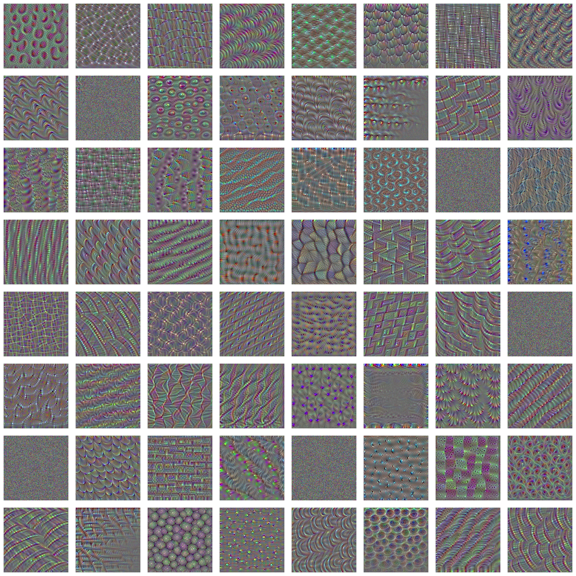
block5_conv1
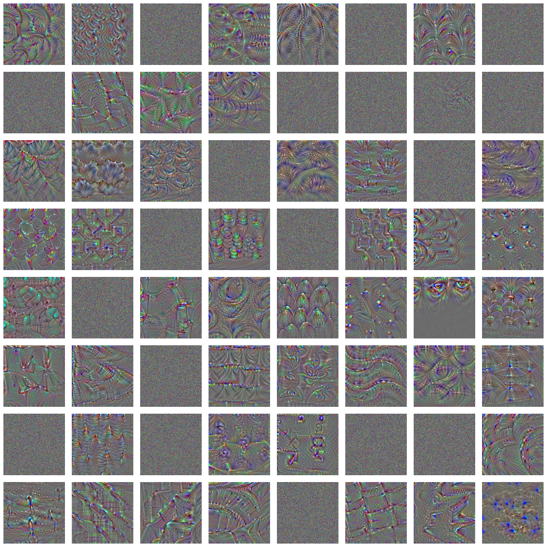
- filters from the
block1_conv1encode simple directional edges and colors (or colored edges in some cases). - filters from
block2_conv1encode simple textures made from combinations of edges and colors. - filters in higher layers begin to resemble textures found in natural images: feathers, eyes, leaves, and so on.
Heatmaps of class activations
This final class activation map (CAM) visualization technique is perhaps the most revealing, in that helps identify which parts of a given image led to a CNN’s classification. In essence, CAM methods consist of producing heatmaps of class activaiton over input images. A class activation heatmap refers to a 2D grid of scores associated with a specific output class. It is computed at every location in an input image, indicating the importance of each location for each class. So in the cats vs dog example, this method would highlight the “cat-like” and “dog-like” locations of each image.
We implement the specific method “Grad-CAM: Visual Explanations from Deep Networks via Gradient-based Localization”. It consists of weighing every channel in the output feature map of a CNN by the gradient of the class with respect to the channel, given some input image. Essentially it creates a spatial map of “how intensely an input image activates a class” by weighing a spatial map of “how intensely each input image activates different channels” by “how importance each channel is with respect to that class”. Again, we demonstrate using VGG16:
#clearing session and loading model with last classification layer
k_clear_session()
model <- application_vgg16(weights = "imagenet")

#processing image for model
img_path <- "files/elephants.jpg"
img <- image_load(img_path, target_size = c(224, 224)) %>%
  image_to_array() %>%  #array of shape (224, 224, 3)
  array_reshape(dim = c(1, 224, 224, 3)) %>% #add batch dim
  imagenet_preprocess_input() #preprocess batch (also channel-wise color normalization)

#predicting class
preds <- model %>% predict(img)
imagenet_decode_predictions(preds, top = 3)[[1]]
## class_name class_description score
## 1 n02504458 African_elephant 0.909421027
## 2 n01871265 tusker 0.086182885
## 3 n02504013 Indian_elephant 0.004354583which.max(preds[1,]) #index of max prediction## [1] 387For the following image, the top 3 classes predicted for this image are:
- African elephant (with 90.9% probability)
- Tusker (with 8.6% probability)
- Indian elephant (with 0.4% probability)
This means the CNN recognized an unknown quantity of African elephants in the image. The index corresponding to the maximally activated “African elephant” class in the prediction vector is 387.
Now to begin visualzing which parts of the image were most “African-elephant” like, we set up the Grad-CAM process:
#extracting elephant entry, output feature map, and gradient for Grad-CAM
african_elephant_output <- model$output[, 387] #AF elephant entry
last_conv_layer <- model %>% get_layer("block5_conv3") #output feature map
grads <- k_gradients(african_elephant_output, last_conv_layer$output)[[1]] #gradient of AF elephant wrt output feature map
pooled_grads <- k_mean(grads, axis = c(1, 2, 3)) #each entry is mean intensity of the gradient over a specific feature map channel, shape (512,)
# function to access the values of `pooled_grads` and the output feature map of `block5_conv3`, given a sample image
iterate <- k_function(list(model$input),
                      list(pooled_grads, last_conv_layer$output[1,,,]))
# values of these two quantities, as arrays, given sample image of 2 elephants
c(pooled_grads_value, conv_layer_output_value) %<-% iterate(list(img))

# multiply each channel in the feature map array by importance wrt to AFE class
for (i in 1:512) {
  conv_layer_output_value[,,i] <-
    conv_layer_output_value[,,i] * pooled_grads_value[[i]]
}
#heatmap of class activation (channelwise mean of resulting feature map)
heatmap <- apply(conv_layer_output_value, c(1,2), mean)

#normalizing heatmap to be between 0 and 1
heatmap <- pmax(heatmap, 0)
heatmap <- heatmap / max(heatmap)

#creating heatmap
write_heatmap <- function(heatmap, filename, width = 224, height = 224,
                          bg = "white", col = terrain.colors(12)) {
  png(filename, width = width, height = height, bg = bg)
  op = par(mar = c(0,0,0,0))
  on.exit({par(op); dev.off()}, add = TRUE)
  rotate <- function(x) t(apply(x, 2, rev))
  image(rotate(heatmap), axes = FALSE, asp = 1, col = col)
}
write_heatmap(heatmap, "images/elephant_heatmap.png")
For reference, we reproduce the original image together with the generated heatmap:
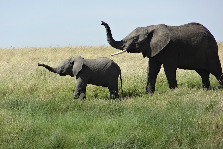
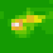
After obtaining the heatmap we see a small area that is maximally activated in the image. Apart from the image, this does not mean much. So now we superimpose the heatmap on the image to precisely identify those areas which are most “African elephant like”:
library(magick) ## Linking to ImageMagick 6.9.9.39
## Enabled features: cairo, fontconfig, freetype, lcms, pango, rsvg, webp
## Disabled features: fftw, ghostscript, x11library(viridis)## Loading required package: viridisLite# Read the original elephant image and it's geometry
image <- image_read(img_path)
info <- image_info(image)
geometry <- sprintf("%dx%d!", info$width, info$height)
# Create a blended / transparent version of the heatmap image
pal <- col2rgb(viridis(20), alpha = TRUE)
alpha <- floor(seq(0, 255, length = ncol(pal)))
pal_col <- rgb(t(pal), alpha = alpha, maxColorValue = 255)
#write_heatmap(heatmap, "images/elephant_overlay.png",
# width = 14, height = 14, bg = NA, col = pal_col) #function discontinued?
# Overlay the heatmap
image_read("files/elephant_overlay.png") %>%
image_resize(geometry, filter = "quadratic") %>%
image_composite(image, operator = "blend", compose_args = "50") %>%
plot() 
One striking realization from this is that the ears of the calf are strongly predictive. In fact, it turns out that one key discrimant between an African and Indian elephant is the shape of their ears. It is truly remarkable that we can extract this sort of information from a CNN.
Summary and practical advice for high-performing models
No matter how organized this material is presented, in its entirety it undoubtedly feels like a whirlwind of disparate and complex ideas tied together under the infamous name Deep Learning. While we have presented much theoretical information to help build intuition when building models, the practical techniques are what begin to separate the amateurs from the professionals. Below we summarize some of the most interesting techniques for ease of reference, along with some terms:
deep learning - subset of machine learning where the model consists of a series of interconnected neural networks; excels in building predictive models with both traditional (tidy) and non-traditional (text, speech, video) data sources.
neural network - a nonlinear function of a linear combination of features: \(Z = \sigma(\alpha_{0} + \alpha^T_X) = \sigma(W^TX)\).
layer - specific variant of a neural network such as alayer_conv2d, layer_global_max_pooling, layer_lstm or layer_dense; fundamental piece that is connected together in a deep learning model.
architecture - refers to the entire deep learning model or network, or in other words to the entire set of hyperparameters in a deep learning model; often given a peculiar name e.g. Xception, VGG19.
Here is a breakdown of where each class of model excels:
- Vector data - densely connected nets.
- Image data - 2D convnets.
- Volumetric data - 3D convnets.
- Sequential data (sound, text, time-series) - 1D convnets or RNNs.
- Video data - 3D convnets or combo of 2D convnet with RNN / 1D convnet.
The traditional workflow for building a deep learning model is as follows:
- Process the data into tensors of appropriate shape.
- Define the deep learning network layer, by layer, where input layer takes tensors of shape equivalent to the input, and the output layer returns data of shape appropriate to the problem.
- Define the problem logistics in the compilation step, e.g. the optimization algorithm, the loss function, and the validation metric.
- Fit the model using training data and labels.
- Evaluate the data on unseen data.
Here is an example of that workflow:
#processing data into tensors of shape n*784
library(keras)
mnist <- dataset_mnist()
train_images <- mnist$train$x
train_labels <- mnist$train$y
test_images <- mnist$test$x
test_labels <- mnist$test$y

train_images <- array_reshape(train_images, c(60000, 28 * 28))
train_images <- train_images / 255
test_images <- array_reshape(test_images, c(10000, 28 * 28))
test_images <- test_images / 255
train_labels <- to_categorical(train_labels)
test_labels <- to_categorical(test_labels)

#defining a simple network: two dense layers
model <- keras_model_sequential() %>%
  layer_dense(units = 512, activation = "relu", input_shape = c(28 * 28)) %>%
  layer_dense(units = 10, activation = "softmax")

#compilation step (defining problem logistics)
model %>% compile(
  optimizer = "rmsprop",
  loss = "categorical_crossentropy",
  metrics = c("accuracy")
)

#fitting the model
history <- model %>% fit(train_images, train_labels, epochs = 5, batch_size = 128)

#evaluating the model
results <- model %>% evaluate(test_images, test_labels, verbose = 0)
predictions <- model %>% predict_classes(test_images[1:10,])
Here are some practical tips:
- processing data into tensors of appropriate shape will require practice, no way around it, especially in text data.
- establish a common-sense baseline before constructing a more complex model.
- downsampling is a necessary technique in CNNs to prevent overfitting; often acheived through pooling layers and strides.
- combo of alternating convolutional and pooling layers allow subsequent layers to see a greater portion of the image, see first CNN example.
layer_separable_conv_2d()is preferred tolayer_conv2din terms of speed and performance, especially when building a model from scratch.
layer_lstmorlayer_gruare highly preferred overlayer_simple_rnndue to the vanishing gradient problem.- data augmentation, regularization, dropout, and batch-normalization are all techniques to prevent overfitting and increase the generalizability of the model; first prevents learning of spurious correlations, second combats correlation between the features, third forces the model to evolve and learn new useful features by zeroing out (sometimes important) output features, and fourth helps propogate the gradient by normalizing the dat at each step.
- visualziing class activations can help identify why certain observations are being misclassified; you can take the misclassified observations and them run them in parallel with a correctly classified observations through the model for further intuition.
- pre-trained bases of popular models can sometimes be useful when constructing a new model, but the success highly depends on the data the previous model was trained on, its success, and the layers which are grabbed from it; try to early layers before the feature maps get increasingly abstract.
- gpus are a must; still fine to use Amazon EC2 instance unless you’re building DL models constantly; really, the instance must be active only during training and maybe data preprocessing; save the model and continue locally once done, only opening to train again; make sure to delete instance, not just stop it or you will be charged.
- practice, practice, practice and have fun; try problems you are sincerely interested in and motivated by assuming data is easily accessible; Kaggle is a great competitive environment for practicing, and it even pays once you are good enough. Two of the most popular liraries are XGBoost or Keras, and they make great use of hyperparameter tuning, avoiding validation-set overfitting, and model ensembling (we’ve discussed the former two in great detail). Happy Learning!!