Think wordyR: nlp in R
Text Analysis
Text (like images or voice recordings), are one of those special data sources which require an entirely different set of computational skills. And with the rise of unstructured text data in nearly every corner of industry, it is imperative for the seasoned data scientist to have considerable ability in dealing with this data.
In this document I’ll survey most of the skills and code needed to process and analyze natural language. This document relies on Tidyverse semantics, specifically those for manipulating strings outlined in Ch.14 of R for Data Science. You can find a more concise reference in the stringr cheatsheet, and a more general understanding of software for NLP in R by surveying the CRAN Task for NLP. My primary resource though was Tidy Text which is an excellent resource for understanding the ins and outs of tidying and analyzing text data in R.
Mechanics
When first faced with text data, the questions I asked myself were:
What code will I use?
How will I structure the data?
What are some useful analytical methods?
How can I visualize it?
Each of the subsequent sections should serve as thorough answers for each of these questions above respectively. More importantly, these questions cover the mechanics of working with text.
String manipulation (stringr in tidyverse)
What code will I use?
In the tidyverse, string manipulation is done primarily through stringr (to avoid inconsistencies in base R’s string methods). This package, together with regular expressions or regexps ( a terse language describing common patterns in strings), supply you with all the tools you’ll to process strings.
Basics
Basically, stringr contains a concise collection of 49 functions for processing strings, and it is built on top of the more comprehensive stringi package consisting of 244 functions. Dig into the source code for any str_function and it’ll be apparent. While the stringr functions are all prefixed by str_, the stringi ones are prefixed by stri_. Before diving into some key functions, let’ talk about strings.
Strings refer to a each single element in a character vector. They are declared like this:
#Mechanics
x <- "Valid string declaration"
y <- 'Also a "valid" declaration' #single quote allows quotes inside a string
z <- c("these", "are", "elements", "of", "a", "string", "vector.")
Practically anything is fair-game inside a string, but things get a little tricky when certain special characters are included. You can view all of these characters via ?"'". While printing a string returns the raw, uninterpreted text, the interpreted version can be viewed through writeLines. For example, consider the raw vs interpreted version of this excerpt from Baudelaire, a poem by Delmore Schwartz.
poem_excerpt## [1] "When I fall asleep, and even during sleep,\r I hear, quite distinctly, voices speaking\r Whole phrases, commonplace and trivial, \r Having no relation to my affairs. \r \r Dear Mother, is any time left to us\r In which to be happy?"writeLines(poem_excerpt)## When I fall asleep, and even during sleep,
I hear, quite distinctly, voices speaking
Whole phrases, commonplace and trivial,
Having no relation to my affairs.
Dear Mother, is any time left to us
In which to be happy?One other strange subtlety worth noting involves regexps. To better explain, consider a simple and exemplary function like str_detect. Like most functions in stringr, it is of the form str_detect(string, pattern, ...). Nothing strange there. But what is happening under the hood when you call this function?
Well, the default behavior of these functions is to interpret the pattern argument as a regexps. This is done by automatically wrapping the string inputted for this argument in a regex call. You can control some finer details of this happens by doing the wrapping yourself, i.e. str_detect(string, regex(pattern, ...)). Regexps have a language all their own, so to gain some familiarity consult the back of the cheat sheet provided in the link. So now that you’re aware of these two strange situations when dealing with special characters or regexps, let’s take a closer look at some functions.
Functions
Here are some fundamental and self-explanatory functions which don’t require a regexps, and some helper functions:
Basics
str_length() - returns the number of characters in a string.
str_c() - combines two or more vectors of strings at the element-level; sep= option defines the character separating tuple-wise concatenations, collapse() option further concatenates tuple-wise concatenations into a single vector.
str_sub() - extracts parts of a string corresponding to inputted first and last position;str_locate() returns starting and end position of every match.
str_sort() - sorts a character vector.
str_order() - returns the order necessary to sort the vector.
regex() - controls finer details of string matching; all str_.() functions are automatically wrapped into a regex() call.
writeLines() - returns string with translated special characters; regular printing prints raw contents.
And here is an example to illustrate some of the jargon above. Guess what will happen then check your answers by executing this code.
str_length(poem_excerpt)

#str_c basics
str_c("x", "y", "z")
str_c("x", NA)
str_c("x", "y", "z", sep = ", ")
str_c("x", "y", "z", collapse = ", ")

#objects of multiple lengths (recycling)
str_c(c("a"), c("b", "c"), c("d" ,"e", "f"))
str_c(c("a"), c("b", "c"), c("d" ,"e", "f"), sep = ", ")
str_c(c("a"), c("b", "c"), c("d" ,"e", "f"), collapse = ", ")

#str_sub basics
x <- c("Apple", "Banana", "Pear")
str_sub(x, 1, 3)
str_sub(x, -3, -1)
str_sub("a", 1, 5)
And now here are the bread and butter tools which make this intuitive way to process strings possible. As a small point, most of these functions have extensions by adding all as a suffix (e.g. str_extract_all) to repeat the function if there are multiple matches within a string in a character vector.
Matching
str_view() - returns illustration of the first match in a string.
str_detect() - returns a logical vector according to whether the pattern is detected.
str_which() - returns the position of any matches.
str_subset() - returns subset of string vector containing matches.
str_extract() - returns first extracted matching piece of string element.
str_match() - returns a character matrix of any matches.
str_count() - returns the number of matches in each string within the character vector.
str_split() - splits a string into pieces by the pattern.
str_replace() - replaces exact matches in a string with new strings.
str_trim() - trims white space from start and end of the string.
str_squish() - trims white space from start and end PLUS any repeated white space within a string.
str_pad() - pads the start and end of string with user input; opposite of str_trim.
Again, here’s some code you can run to get a better feel for these functions.
#example vector
x <- c("Apple", "Banana", "Pear", " coco   nut ")

#matches
str_detect(x, "Banana")
str_which(x, "Pear")
str_subset(x, "e")
str_extract(x, "e")
str_match(x, "e")
str_count(x, "a")

#other uses
str_split(x, "a")
str_replace(x, "a", "q")
str_replace_all(x, "a", "q")
str_trim(x)
str_squish(x)
str_pad(x, 8, "left", "Z")
Below are some of the basic regexps tips to find matches. anchors ^ $ match beginning and end of string respectively, both match complete string; str_view_all() returns illustration of all matches in a string; character classes and alternatives facilitate matching; number of matches may be controlled through ?, +, and * (0-1, 1 or more, 0 or more).
Data formats
How will I structure the data?
Tidy format (explained below) is usually sufficient for most text analysis. But some tasks or packages require data to be in other formats, most notably a corpus or document-term matrix. In this section we’ll cover what each structure is useful for, and how you can covert between them. Here is a helpful visual.
From the visual we see that all of these text structures are amenable to analysis and visualizations. The reason why these different structures exist is because certain packages and methods only work with certain structures. Let’s quickly define the other two data structures:
- Tidy: one token per row, with meta data for that token describing each token in data frame.
- Corpus: designed to store document collections before tokenization in a corpus; typically raw strings annotated with additional meta-data and details such as id, date/time, language, or title.
- Document-term matrix: sparse matrix describing a corpus of documents with one row for each document, one row per term (word), and each value representing some summary measure like word-count or the td-idf statistic.
Let’s briefly spend some time understanding each of these three structures:
Tidy format
Per Hadley Wickham, tidy data satisfies these criteria:
- Each variable is a column.
- Each observation is a row.
- Each type of observational unit is a token
In Tidy Text the authors extend the concept of tidy data to text, and define the tidy text format as being a table with one-token-per-row, where a token can be a word, sentence, paragraph, or other meaningful token of text. Ordinarily the tidy text format is sufficient to carry-out a text analysis. One key function which underpins making data tidy is:
unnest_tokens- breaks down text into a tidy format by the user-requested type of token; default is tokenizing words, but other options include characters, n-grams, sentences, lines, paragraphs, or separation around a regex.
As a simple example, we tidy the text below like so:
text <- c("Because I could not stop for Death -",
          "He kindly stopped for me -",
          "The Carriage held but just Ourselves -",
          "and Immortality")
text_df <- tibble(line = 1:4, text = text)
text_df %>%
  unnest_tokens(word, text)
## # A tibble: 20 x 2
## line word
## <int> <chr>
## 1 1 because
## 2 1 i
## 3 1 could
## 4 1 not
## 5 1 stop
## 6 1 for
## 7 1 death
## 8 2 he
## 9 2 kindly
## 10 2 stopped
## 11 2 for
## 12 2 me
## 13 3 the
## 14 3 carriage
## 15 3 held
## 16 3 but
## 17 3 just
## 18 3 ourselves
## 19 4 and
## 20 4 immortalityIn a more realistic example, we could leverage some of the online resources available for getting full texts such as janeaustenr, gutenbergr or many others to tidy text:
#text before tidying
austen_books()
## # A tibble: 73,422 x 2
## text book
## * <chr> <fct>
## 1 "SENSE AND SENSIBILITY" Sense & Sensibility
## 2 "" Sense & Sensibility
## 3 "by Jane Austen" Sense & Sensibility
## 4 "" Sense & Sensibility
## 5 "(1811)" Sense & Sensibility
## 6 "" Sense & Sensibility
## 7 "" Sense & Sensibility
## 8 "" Sense & Sensibility
## 9 "" Sense & Sensibility
## 10 "CHAPTER 1" Sense & Sensibility
## # … with 73,412 more rows#formatting text
tidy_books <- austen_books() %>%
group_by(book) %>%
mutate(linenumber = row_number(),
chapter = cumsum(str_detect(text, regex("^chapter [\\divxlc]",
ignore_case = TRUE)))) %>%
ungroup()
#tidying text
books <- tidy_books %>%
unnest_tokens(word, text) %>%
anti_join(stop_words) #removes "trivial" words
books## # A tibble: 217,609 x 4
## book linenumber chapter word
## <fct> <int> <int> <chr>
## 1 Sense & Sensibility 1 0 sense
## 2 Sense & Sensibility 1 0 sensibility
## 3 Sense & Sensibility 3 0 jane
## 4 Sense & Sensibility 3 0 austen
## 5 Sense & Sensibility 5 0 1811
## 6 Sense & Sensibility 10 1 chapter
## 7 Sense & Sensibility 10 1 1
## 8 Sense & Sensibility 13 1 family
## 9 Sense & Sensibility 13 1 dashwood
## 10 Sense & Sensibility 13 1 settled
## # … with 217,599 more rowsNotice that at the end, each data set is split into one-token per row, and that our tools with handling strings helped us extract useful meta-data by which we can better describe any particular token. This is pretty much all there is to tidying data. We’ll touch on this in the other sections as we go over how to tidy each of the other formats.
Corpus format
Corpus objects are a convenient way to store collections of documents, especially for use with the tm package. Collections of documents can even be written using writeCorpus for later use. Corpus objects are essentially lists with additional attributes. Each item along with the entire corpus has both metadata and content.
data("acq")
acq
## <<VCorpus>>
## Metadata: corpus specific: 0, document level (indexed): 0
## Content: documents: 50acq[[1]]## <<PlainTextDocument>>
## Metadata: 15
## Content: chars: 1287As is corpus objects cannot be analyzed, but they can be converted into regular text data via tidy, which can then be made into tidy text via unnest_tokens. When tidied, metadata becomes columns alongside the text and everything after that point is a traditional text analysis. For example, we can tidy a corpus and count the most frequent words in each article like so:
acq %>% tidy %>%
  select(-places) %>%
  unnest_tokens(word, text) %>%
  anti_join(stop_words, by = "word") %>%
  count(word, sort = TRUE)
## # A tibble: 1,566 x 2
## word n
## <chr> <int>
## 1 dlrs 100
## 2 pct 70
## 3 mln 65
## 4 company 63
## 5 shares 52
## 6 reuter 50
## 7 stock 46
## 8 offer 34
## 9 share 34
## 10 american 28
## # … with 1,556 more rowsGoing the other way we can create a document-term matrix through DocumentTermMatrix (or a term-document matrix via TermDocumentMatrix). Both of these employ sparse matrices for corpora, whereas as.matrix would store them in very dense, memory-intensive matrices. To illustrate how robust tidy is to the different data formats, let’s tidy another version of a corpus object in the quanteda package:
data("data_corpus_inaugural", package = "quanteda")
summary(data_corpus_inaugural)
## Length Class1 Class2 Mode
## 58 corpus character characterdata_corpus_inaugural %>% tidy## # A tibble: 58 x 5
## text Year President FirstName Party
## <chr> <int> <chr> <chr> <fct>
## 1 "Fellow-Citizens of the Senate and o… 1789 Washington George none
## 2 "Fellow citizens, I am again called … 1793 Washington George none
## 3 "When it was first perceived, in ear… 1797 Adams John Federalist
## 4 "Friends and Fellow Citizens:\n\nCal… 1801 Jefferson Thomas Democratic-…
## 5 "Proceeding, fellow citizens, to tha… 1805 Jefferson Thomas Democratic-…
## 6 "Unwilling to depart from examples o… 1809 Madison James Democratic-…
## 7 "About to add the solemnity of an oa… 1813 Madison James Democratic-…
## 8 "I should be destitute of feeling if… 1817 Monroe James Democratic-…
## 9 "Fellow citizens, I shall not attemp… 1821 Monroe James Democratic-…
## 10 "In compliance with an usage coeval … 1825 Adams John Qui… Democratic-…
## # … with 48 more rowsIn a final example of tidying Corpus data for analysis, we could use the tm.plugin.webmining package to retrieve the 20 most recent articles related to a certain stock. Let’s take a look at 8 healthcare companies:
company <- c("Johnson & Johnson", "Pfizer", "Novartis", "Merck & Co.",
            "Abbvie", "Abbott Laboratories", "Takeda Pharmaceutical Co Ltd")
symbol <- c("JNJ", "PFE", "NVS", "MRK", "ABBV", "ABT", "TAK")

download_articles <- function(symbol) {
  WebCorpus(GoogleFinanceSource(paste0("NYSE:", symbol)))
}

stock_articles <- tibble(company = company,
                             symbol = symbol) %>%
  mutate(corpus = map(symbol, download_articles))
Document-term matrix format
Document-term matrices are a popular data format for text mining formats where:
- each row represents one document (e.g. book, article).
- each column represents one term.
- each value (typically) contains how many times that term appeared in the document.
Let’s look at an example of a DocumentTermMatrix object defined by the tm package.
data("AssociatedPress", package = "topicmodels")What we see is that the data set contains 2246 documents (each an AP article) with 10473 terms (distinct words). The fact that the DTM is 99% sparse implies that 99& of the word-document pairs are zero. In other words, in this matrix where every row is a document and every column a word from the collection of unique words shared across all documents, only 1% of cells are non-zero. This doesn’t really translate well into a comment about the similarity of the documents, so we’ll leave it at that. To look into the actual terms we can use Terms
head(Terms(AssociatedPress))## [1] "aaron" "abandon" "abandoned" "abandoning" "abbott"
## [6] "abboud"The quanteda package also has their own implementation of DTM through their dfm (document-feature matrix) object. Let’s look at an example of one:
data("data_corpus_inaugural", package = "quanteda") #corpus object
quanteda::dfm(data_corpus_inaugural, verbose = FALSE)
## Document-feature matrix of: 58 documents, 9,360 features (91.8% sparse) and 4 docvars.
## features
## docs fellow-citizens of the senate and house representatives :
## 1789-Washington 1 71 116 1 48 2 2 1
## 1793-Washington 0 11 13 0 2 0 0 1
## 1797-Adams 3 140 163 1 130 0 2 0
## 1801-Jefferson 2 104 130 0 81 0 0 1
## 1805-Jefferson 0 101 143 0 93 0 0 0
## 1809-Madison 1 69 104 0 43 0 0 0
## features
## docs among vicissitudes
## 1789-Washington 1 1
## 1793-Washington 0 0
## 1797-Adams 4 0
## 1801-Jefferson 1 0
## 1805-Jefferson 7 0
## 1809-Madison 0 0
## [ reached max_ndoc ... 52 more documents, reached max_nfeat ... 9,350 more features ]While both of these formats are necessary to utilize some of the tools in each of these packages, both DTMs and DFMs can be converted to tidy text through tidy if needed as well:
ap_td <- AssociatedPress %>% tidy
ap_td
## # A tibble: 302,031 x 3
## document term count
## <int> <chr> <dbl>
## 1 1 adding 1
## 2 1 adult 2
## 3 1 ago 1
## 4 1 alcohol 1
## 5 1 allegedly 1
## 6 1 allen 1
## 7 1 apparently 2
## 8 1 appeared 1
## 9 1 arrested 1
## 10 1 assault 1
## # … with 302,021 more rowsquanteda::dfm(data_corpus_inaugural, verbose = FALSE) %>% tidy## # A tibble: 44,710 x 3
## document term count
## <chr> <chr> <dbl>
## 1 1789-Washington fellow-citizens 1
## 2 1797-Adams fellow-citizens 3
## 3 1801-Jefferson fellow-citizens 2
## 4 1809-Madison fellow-citizens 1
## 5 1813-Madison fellow-citizens 1
## 6 1817-Monroe fellow-citizens 5
## 7 1821-Monroe fellow-citizens 1
## 8 1841-Harrison fellow-citizens 11
## 9 1845-Polk fellow-citizens 1
## 10 1849-Taylor fellow-citizens 1
## # … with 44,700 more rowsIts worth reminding that when we are dealing with DTM/DFMs, tidy only gets us to summarized text; there is no way to get back to tidy text from here. Still, there is plenty of analysis we can do with summarized data. If we wanted to go back the other way from summarized data back to a DTM or DFM, we could use cast_dtm or cast_dfm respectively. There is even a sparse matrix from the Matrix package that we can apply:
ap_td %>% cast_dtm(document, term, count)## <<DocumentTermMatrix (documents: 2246, terms: 10473)>>
## Non-/sparse entries: 302031/23220327
## Sparsity : 99%
## Maximal term length: 18
## Weighting : term frequency (tf)ap_td %>% cast_dfm(document, term, count)## Document-feature matrix of: 2,246 documents, 10,473 features (98.7% sparse).
## features
## docs adding adult ago alcohol allegedly allen apparently appeared arrested
## 1 1 2 1 1 1 1 2 1 1
## 2 0 0 0 0 0 0 0 1 0
## 3 0 0 1 0 0 0 0 1 0
## 4 0 0 3 0 0 0 0 0 0
## 5 0 0 0 0 0 0 0 0 0
## 6 0 0 2 0 0 0 0 0 0
## features
## docs assault
## 1 1
## 2 0
## 3 0
## 4 0
## 5 0
## 6 0
## [ reached max_ndoc ... 2,240 more documents, reached max_nfeat ... 10,463 more features ]ap_td %>% cast_sparse(document, term, count) %>% dim## [1] 2246 10473Having covered all of these, we should now be able to go from text to DTM/DFM to summarized text, text to tidy text so summarized text, and from corpus objects to either text or DTM/DFM. This blows our arsenal wide open in terms of the tools we can now use to analyze text in R.
Analysis methods
Several statistical methods lend themselves well to the tidy text framework developed in this book. Four methods are touched on to give someone a nice start in text analysis:
- term frequency - frequency of which a word appears; extends to n-grams.
- tf-idf - statistic used to measure the importance of a term in a document relative to other documents; identifies words which characterize a document relative to other documents.
- correlations - measures how often words appear together in a particular document.
- topic modeling - unsupervised classification method to group documents into certain groups which may represent topics; basically Latent Dirichlet allocation (LDA).
- sentiment analysis - measures the sentiment in a document.
Let’s take a little whirlwind tour through the methods.
Term frequency
Its exactly what it sounds like: the proportion of times a word appears in a document relative to the total count. Calculating it is incredibly simple using tidy tools. Let’s use the tidied Jane Austen books from previous and get the term frequency of words across books(pay special attention to removing stop words, as these will unduly appear more often than other terms):
book_words  <- austen_books() %>%
  unnest_tokens(word, text) %>%
  anti_join(stop_words) %>%
  count(book, word, sort = T)
total_words <- book_words %>%
  group_by(book) %>%
  summarize(total = sum(n))

book_words <- book_words %>%
  left_join(total_words) %>%
  mutate(tf = n / total)
book_words
## # A tibble: 37,224 x 5
## book word n total tf
## <fct> <chr> <int> <int> <dbl>
## 1 Mansfield Park fanny 816 47968 0.0170
## 2 Emma emma 786 46775 0.0168
## 3 Sense & Sensibility elinor 623 36330 0.0171
## 4 Emma miss 599 46775 0.0128
## 5 Pride & Prejudice elizabeth 597 37246 0.0160
## 6 Mansfield Park crawford 493 47968 0.0103
## 7 Sense & Sensibility marianne 492 36330 0.0135
## 8 Persuasion anne 447 25488 0.0175
## 9 Mansfield Park miss 432 47968 0.00901
## 10 Northanger Abbey catherine 428 23802 0.0180
## # … with 37,214 more rowsTerm-frequency inverse document-frequency (Tf-idf)
Let \(n_1\) be the number of documents, \(n_2\) be the number of documents containing the term, \(w_1\) be the number of times a word appears in a document, and \(w_{total}\) the total number of words in a document. Then for any given term, it’s tf-idf is:
\[ \frac{w_1}{w_{total}} \times ln\bigg(\frac{n_1}{n_2}\bigg) \]
where the second term is the inverse-document frequency. Looking at the second term we see that \(idf \in [0,\infty)\), where 0 occurs if the term is found in all documents. This means that the whole statistic basically weighs the term frequency by how rare it is relative to other documents. The rarer it is, the relatively larger the weight.
To compute this we return to the previous example and use the super convenient bind_tf_idf function. As a good sanity check you could multiply tf by idf:
book_words %>%
  bind_tf_idf(word, book, n)
## # A tibble: 37,224 x 7
## book word n total tf idf tf_idf
## <fct> <chr> <int> <int> <dbl> <dbl> <dbl>
## 1 Mansfield Park fanny 816 47968 0.0170 0.693 0.0118
## 2 Emma emma 786 46775 0.0168 1.10 0.0185
## 3 Sense & Sensibility elinor 623 36330 0.0171 1.79 0.0307
## 4 Emma miss 599 46775 0.0128 0 0
## 5 Pride & Prejudice elizabeth 597 37246 0.0160 0.693 0.0111
## 6 Mansfield Park crawford 493 47968 0.0103 1.79 0.0184
## 7 Sense & Sensibility marianne 492 36330 0.0135 1.79 0.0243
## 8 Persuasion anne 447 25488 0.0175 0.182 0.00320
## 9 Mansfield Park miss 432 47968 0.00901 0 0
## 10 Northanger Abbey catherine 428 23802 0.0180 0.693 0.0125
## # … with 37,214 more rowsTo display the words which characterize a document Tidy Text uses bar-plots but that misses the point and implicitly drives attention to the numbers which is surely not the intention. Faceted word-clouds might be more effective here, maybe even of a timeline for publishing. Point is, its possible to translate this insight visually.
Correlations
In a text context, correlation refers to how often words appear together vs not. Ordinarily it captures similarity in how to two things are changing, but in text its more so looking at words which appear together within a certain window. To begin looking at this we split Pride and Prejudice into 10-line sections and use widyr::pairwise_count:
austen_section_words <- austen_books() %>%
  filter(book == "Pride & Prejudice") %>%
  mutate(section = row_number() %/% 10) %>%
  filter(section > 0) %>%
  unnest_tokens(word, text) %>%
  filter(!word %in% stop_words$word)

austen_section_words %>%
  pairwise_count(word, section, sort = T)
## # A tibble: 796,008 x 3
## item1 item2 n
## <chr> <chr> <dbl>
## 1 darcy elizabeth 144
## 2 elizabeth darcy 144
## 3 miss elizabeth 110
## 4 elizabeth miss 110
## 5 elizabeth jane 106
## 6 jane elizabeth 106
## 7 miss darcy 92
## 8 darcy miss 92
## 9 elizabeth bingley 91
## 10 bingley elizabeth 91
## # … with 795,998 more rowsFrom this we should see that looking at correlation might not be too insightful since “Elizabeth” and “Darcy” are also one of the most common individual words. Instead we could use the phi coefficient to look at correlation, since it focuses on how often a pair of words both appears together or are absent together, relative to times they appear without the other. So if we imagine a contingency table for any two sets of words, then:
\[ \phi(x, y) = \frac{n_{11}n_{00}-n_{10}n_{01}}{\sqrt{n_1n_0n_0n_1}} \]
Computing this term is pretty easily done using widyr::pairwise_cor:
austen_section_words %>%
  group_by(word) %>%
  filter(n() >= 20) %>%  #filter to relatively common words first
  pairwise_cor(word, section, sort = T) %>%
  slice(seq(1, nrow(.), 2))
## # A tibble: 77,421 x 3
## item1 item2 correlation
## <chr> <chr> <dbl>
## 1 bourgh de 0.951
## 2 pounds thousand 0.701
## 3 william sir 0.664
## 4 catherine lady 0.663
## 5 forster colonel 0.622
## 6 fitzwilliam colonel 0.543
## 7 de catherine 0.360
## 8 uncle aunt 0.353
## 9 hour half 0.344
## 10 bourgh catherine 0.322
## # … with 77,411 more rowsA word network is a solid choice for visualizing correlations, but unless there’s something particularly insightful, it might be best to use this as more of an exploratory step.
Topic Modeling
Topic modeling is performed through LDA here. Basically, the idea is to find a natural grouping for documents based on probabilities. Going into the math of it is beyond the scope of this review, but we will focus on how to implement it in R. Basically the model is based on the ideas that:
- everu document is a mixture of topics.
- every topic is a mixture of words.
LDA statistically estimates both of these simultaneously. Fitting the model is quite easy, most of the work revolves around interpreting the model. To illustrate this we’ll start with the DTM example we used previously:
ap_lda <- LDA(AssociatedPress, k = 2, control = list(seed = 1234))
ap_lda
## A LDA_VEM topic model with 2 topics.In this model, \(\beta\) represents per-topic, per-word probabilities. We can extract these using tidy. At that point we can look at other values with meaningful interpretations such as \(log(\frac{\beta_1}{\beta_2})\).
ap_lda %>%
  tidy(matrix = "beta") %>%
  mutate(topic = paste0("topic", topic)) %>%
  spread(topic, beta) %>%
  filter(topic1 > .001, topic2 > .001) %>%
  mutate(log_ratio = log2(topic2 / topic1))
## # A tibble: 49 x 4
## term topic1 topic2 log_ratio
## <chr> <dbl> <dbl> <dbl>
## 1 american 0.00203 0.00168 -0.270
## 2 back 0.00125 0.00103 -0.284
## 3 city 0.00167 0.00128 -0.385
## 4 day 0.00178 0.00148 -0.264
## 5 department 0.00188 0.00100 -0.905
## 6 economic 0.00103 0.00111 0.115
## 7 federal 0.00205 0.00142 -0.531
## 8 first 0.00262 0.00242 -0.110
## 9 five 0.00109 0.00107 -0.0250
## 10 four 0.00103 0.00125 0.280
## # … with 39 more rowsAt this point we could illustrate the topics, actually quite similar to the tf-idf statistic. Since LDA is essentially giving us words which characterize documents, we could use barplots to illustrate these differences like the book does. Again, my suggestion is to use something more illustrative of the differences between these topics such as a modified word cloud. Any further insight requires a better understanding of the underlying theory, so this is a good place to stop.
Sentiment Analysis
This is not so much a general technique, but more so a type of analysis that is popular with text. And since there are tidy tools which lend themselves well to this, I think its good to touch on.
Much of this is possible because tidytext contains several sentiment lexicons within its sentiments data set. It’s three general purpose sentiment lexicons are:
AFINNfrom Finn Arup Nielsen.
bingfrom Bing Liu et al.
nrcfrom Saif Mohammad and Peter Turney.
sentiments can be accessed through tidytext, and particular lexicons can be acquired through get_sentiments:
tidytext::sentiments #default to bing## # A tibble: 6,786 x 2
## word sentiment
## <chr> <chr>
## 1 2-faces negative
## 2 abnormal negative
## 3 abolish negative
## 4 abominable negative
## 5 abominably negative
## 6 abominate negative
## 7 abomination negative
## 8 abort negative
## 9 aborted negative
## 10 aborts negative
## # … with 6,776 more rowsget_sentiments("nrc") #biggest## # A tibble: 13,901 x 2
## word sentiment
## <chr> <chr>
## 1 abacus trust
## 2 abandon fear
## 3 abandon negative
## 4 abandon sadness
## 5 abandoned anger
## 6 abandoned fear
## 7 abandoned negative
## 8 abandoned sadness
## 9 abandonment anger
## 10 abandonment fear
## # … with 13,891 more rowsKeep in mind that words carry different sentiment in different contexts, e.g. share (noun) in finance is neutral vs share (verb) is generally positive. Really the only tool needed to begin a sentiment analysis is inner_join to map words in a document to a sentiment. At that point the analysis is up to our imagination. Using the Jane Austen books we tidied in the Tidy Format section, we can obtain a simple sentiment score like this:
books %>%
  inner_join(get_sentiments("bing")) %>%
  count(book, index = linenumber %/% 80, sentiment) %>%
  spread(sentiment, n, fill = 0) %>%
  mutate(sentiment = positive - negative)
## Joining, by = "word"## # A tibble: 920 x 5
## book index negative positive sentiment
## <fct> <dbl> <dbl> <dbl> <dbl>
## 1 Sense & Sensibility 0 16 26 10
## 2 Sense & Sensibility 1 19 44 25
## 3 Sense & Sensibility 2 12 23 11
## 4 Sense & Sensibility 3 15 22 7
## 5 Sense & Sensibility 4 16 29 13
## 6 Sense & Sensibility 5 16 39 23
## 7 Sense & Sensibility 6 24 37 13
## 8 Sense & Sensibility 7 22 39 17
## 9 Sense & Sensibility 8 30 35 5
## 10 Sense & Sensibility 9 14 18 4
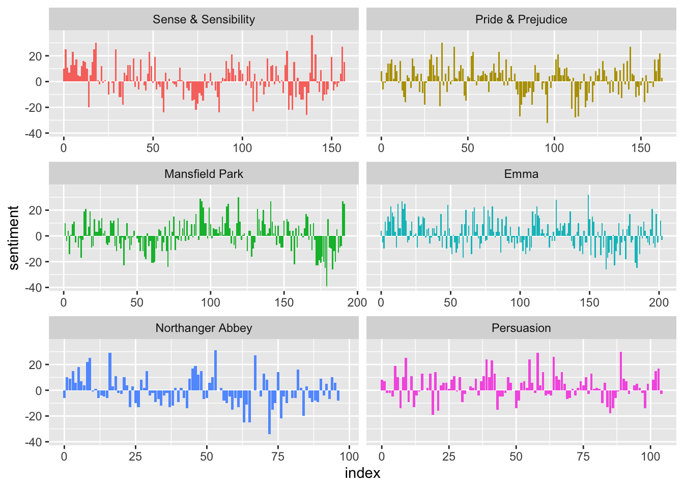
## # … with 910 more rowsSee the visualization section to see a good illustration of sentiment over time. As a word of caution about the use of a sentiment dictionary, I thought I would include a very poignant visual:
What this shows is that while some general trends exist, there is considerable variability across dictionaries. So one should not rush to conclusions when seeing anything like this, because the strength of the conclusion heavily depends upon the quality of the data, i.e. sentiment dictionary.
Visualization
Illustrating insight from text is still very much a work in progress. Nonetheless, there are some very poignant plots which really get a message across. Instead of going through some of the visualizations systematically, I’ll simply recreate some of the ones I found interesting, as well as some which are wholly unique to text analysis.
First there is an incredibly useful and poignant faceted plot that allows us to look at how the frequency of certain words change over time:
Another use of time is in examining how the sentiment of a document varies across time, where we could bin the book into 80 line sections of Jane Austen novels:
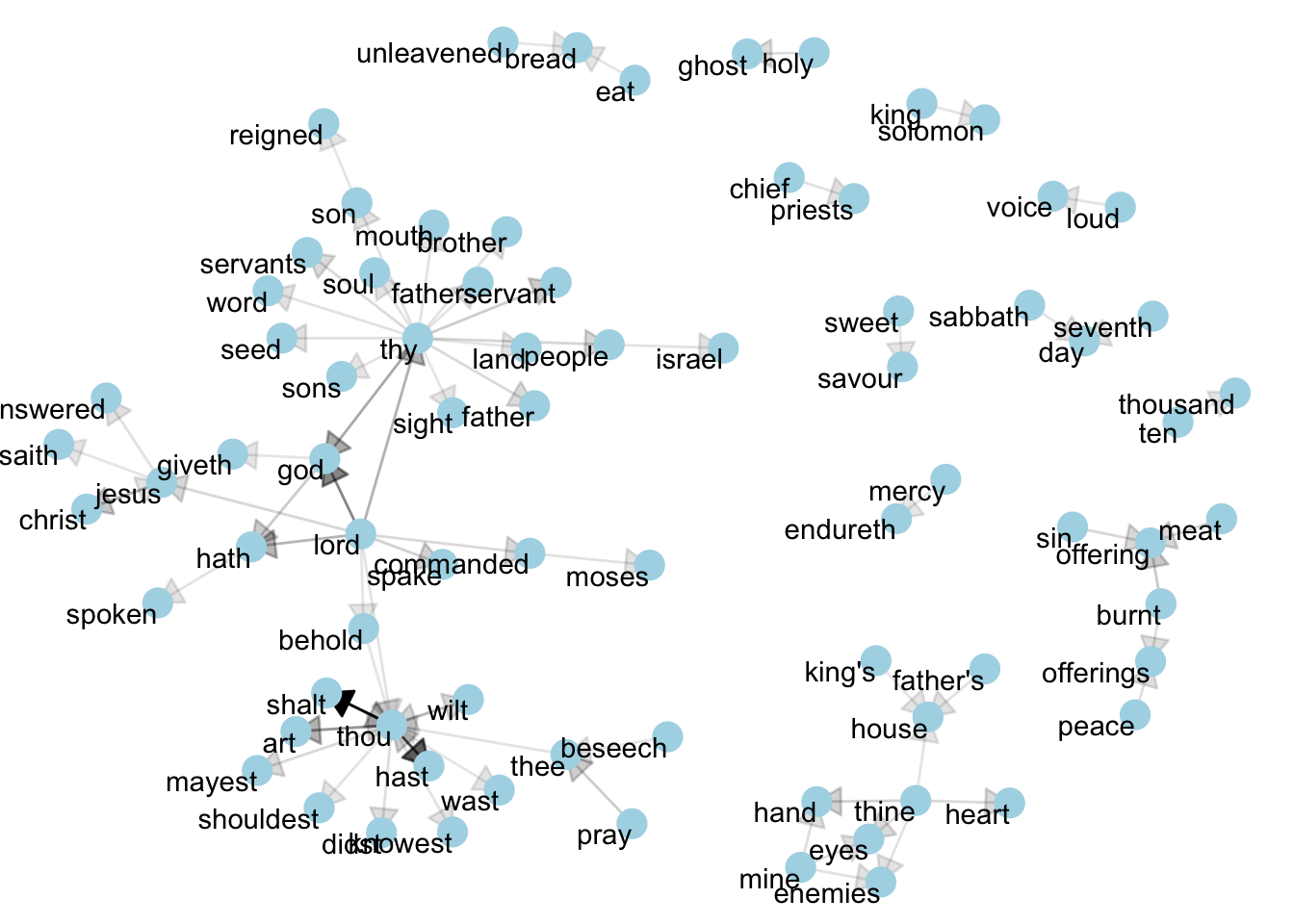
Besides these plots, many text analyses are riddled with bar plots which are not all that effective. The rest of the plots I’ll show are ones unique to text analyses. First is a word network that is a nice one-hit display of n-grams which occur at least x times. Its a nice start to start looking at relationships between words and themes. Below we look at bi grams in book 10 of the King James Bible occurring at least 40 times:
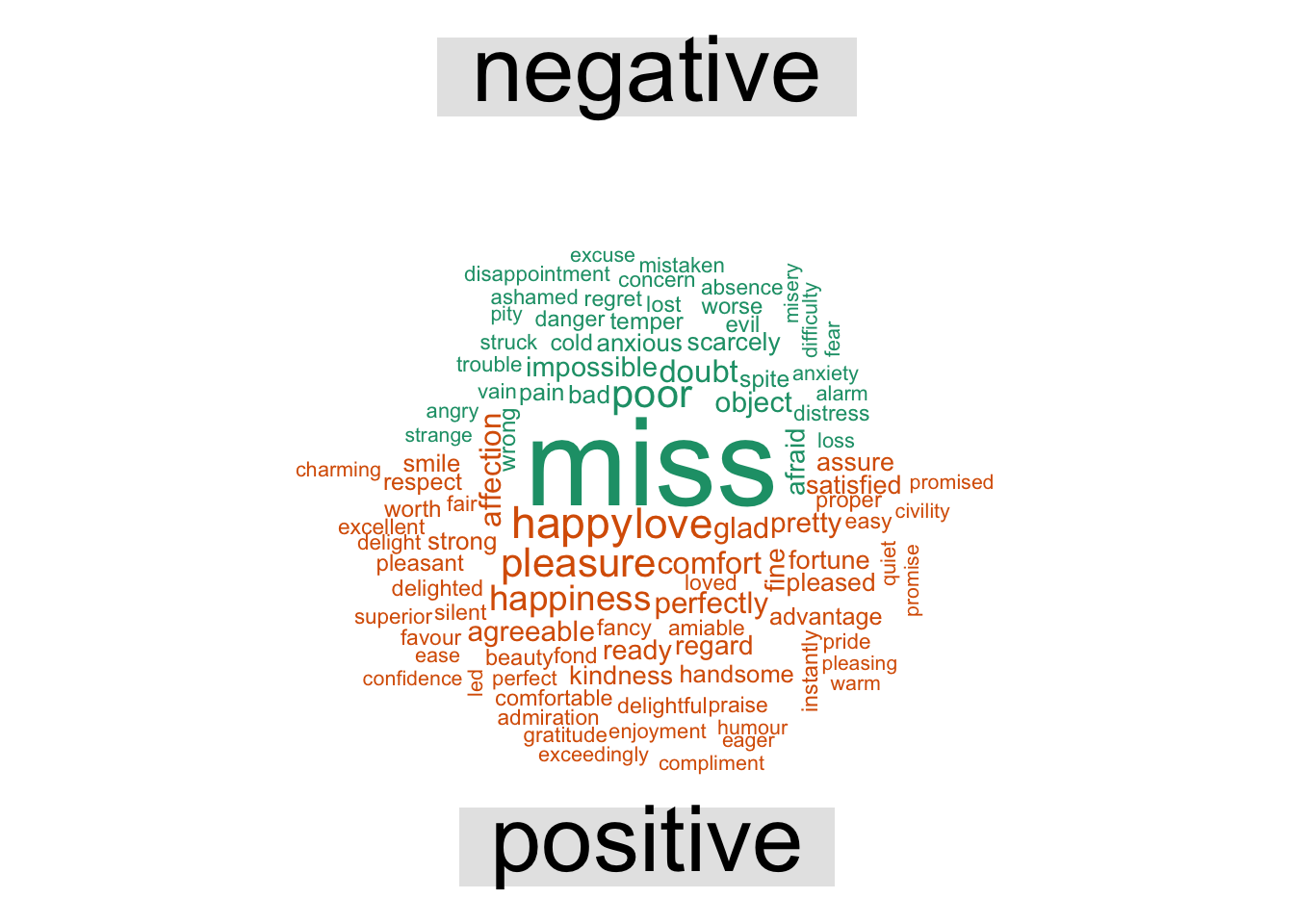
Returning back to sentiment, word clouds are good to examine the frequencies at which words appear. We could also use it to compare frequencies of two groups or documents. In the example below we’ll look a word cloud to find the most common positive and negative words in the Jane Austen novels:
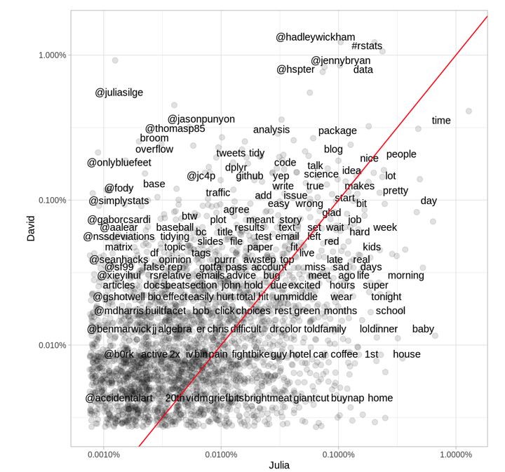
One last visualization which works on some levels is basically a scatter plot where the data is tokens (usually words) shared between two documents. Each axes measures the frequency at which a word appears for each document. Its provides a useful comparison between two documents on the word level. For example, we can look at the twitter use of the two authors of Tidy Text.
Visualizing text is not easy, but using some of the ideas illustrated in the previous plots we can see that it is possible to share some of our insight from text with others. There is definitely room for improvement, but we have some nice ideas here.
Conclusion
Of all the different forms in which data may exist (e.g. numeric, functions, images), text is easily the most abundant and easily attainable. From this it follows that there is a wealth of insight in the mounds of unstructured data online or within walls of privacy like companies. These tools above allow us to start working on and learning from text in a tidy way. To dive deeper into the world of NLP in R, please refer to the corresponding CRAN Task View, and to the NLP Wiki page to view the breadth of tasks in this field.