Breaking it down with PCA

September 7, 2017 9 minutes read

statistics • unsupervised • machine learning

Motivation

PCA (principal component analyses) simultaneously refers to the process for computing PC’s, and the use PC’s to explore and understand the data. Principal components refer to a smaller number of representative variables which collectively explain most of the variability in the orginal set of (usually large and correlated) variables. In other words, the principal components of a data set serve as a low-dimensional representation of it, capturing the greatest amount of variation.

PCA’s utility lies in its ability to reduce. Often, the signal in the data is concentrated within the 1st few principal components, making PCA an effective dimension-reduction tool. This resultant data set consisting of principal components is valuable for many statistical problems, e.g. regression, classification, and clustering. PCA is also useful in visualizing high-dimensional data, sometimes revealing interesting patterns e.g. clusters. Strap on, it’s getting bumpy.

Idea, Definitions, and Notations

For covariates $\mathbf{X_1,...X_p}$, the first principal component is the normalized linear combination of features, \[ \mathbf{Z_1=u_{11}X_1 + u_{21}X_2 +...+u_{p1}X_p} \] containing the largest variance, and subject to the constraint that $\sum_{j=1}^p{u_{j1}^2=1}$. Here, $\mathbf{u_{11},...,u_{p1}}$ represent the loadings of the 1st principal component, and $\mathbf{Z_1,...,Z_n}$ represent the scores of the 1st principal component. An interpretation of these two concepts will be provided briefly.

To illustrate how the principal components are computed, we will calculate the first two principal components. First, we must center all the variables, i.e. $\mathbf{X^c} = (X_1-\bar{X}_1,X_2-\bar{X}_2,...,X_p-\bar{X}_p)$. Centering the variables reduces the values into standard deviations, which becomes the variance later on when they are squared in the objective function. Next, to look for linear combinations of the form: \[ z_{i1}=u_{11}x_{i1} + u_{21}x_{i2} +...+u_{p1}x_{ip} \] subject to the above constraint, we solve this objective function which has 1 equation, and 1 unknown via an eigen-decomposition: \[ \mathbf{\frac1n\sum_{i=1}^nz_{i1}^2 =\max_{u_{11},..,u_{1p}} \left\{ \frac1n\sum_{i=1}^n(\sum_{j=1}^p{u_{j1}x_{ij})^2)}\right\}}\quad subject\: to\: \mathbf{\sum_{j=1}^p{u_{ji}^2 =1}} \] An important point is that since $1/n\sum_{i=1}^nx_{ij}=0$, then $1/n\sum_{i=1}^nz_{i1}^2=0$, i.e. the average of the first principal component equals zero. Thus, the objective function above maximizes the sample variance of the $n$ values of $z_{i1}$. Likewise, the second principal component represents a linear combination of $X_1,...X_p$ with the highest variance of all linear combinations, with the additional constraint that it is uncorrelated with $Z_1$, which to turns out to imply orthogonality between the direction of $u_2$ and $u_1$. Similarly, it takes the form: \[ z_{i2}=u_{12}x_{i1} +u_{22}x_{i2} +...+u_{p2}x_{ip} \] Each subsequent principal component is uncorrelated with those before it, the $Var(Z_i)<Var(Z_j)$ for all $i<j$, and the maximum number of principal components ($min(n-1,p)$) captures all of the variability.

To illustrate how the solution would actually be computed, we now introduce the same material in matrix notation.

Prior to introducing PCA, we must introduce SVD (singluar value decomposition); a decomposition underpinning PCA. Assume matrix $\mathbf{\underset{Nxp}{\mathrm{X}}}$ is centered, i.e. $\mathbf{\underset{Nxp}{\mathrm{X}}\leftarrow (X-\bar{X})}$. SVD of $X$ has the form: \[ \mathbf{X=USV^T=\sum_{k=1}^{n}u_ks_kv_k^T} \quad where, \] $\mathbf{\underset{Nxp}{\mathrm{U}}}$ has columns spanning the column space of $\mathbf{X}$, whose columns $u_j$ are called the left singular vectors.
$\mathbf{\underset{pxp}{\mathrm{V}}}$ has columns spanning the row space of $\mathbf{X}$, whose columns $v_j$ are called the right singular vectors.
Both $U$ and $V$ are orthogonal, e.g. $A^TA=I$, and

$\mathbf{S}$ is a $p\times p$ diagonal matrix whose diagonal elements $s_1>s_2>...>s_p\geq0$ are called the singular values of $X$. If $\exists s_j=0$, $\mathbf{X}$ is singular.

Keeping this in the back of our mind, we can now forumalate PCA. To rehash, the principal components of $\mathbf{X}$ in $\Re^p$ provide a sequence of best linear approximations of $\mathbf{X}$, all of ranks $q\leq p$. Mathematically said, for observations $x_1,x_2,...,x_N$, the rank-q linear model representing them is: \[ f(\lambda) = \mu + \mathbf{V}_q\lambda, \quad where \] $\mu$ is a location vector in $\Re^p$
$\mathbf{V}_q$ is a $p\times q$ orthonormal matrix, and
$\lambda$ is a $q$ vector of parameters.

Developing the last perspective a bit further, PCA can be conceptualized as a linear model, or more specifically a parametric representation of an affine hyperplane of rank q. To fit this model by least squares amounts to minimizing the reconstruction error: \[ \min_{\mu, {\lambda_i}, \mathbf{V}_q} \sum_{i=1}^N{||x_i-\mu-\mathbf{V}_q\lambda_i||^2},\quad or\ eqivalently \] \[ \min_{S,U,V}\frac 12{||\mathbf{X} -\mathbf{USV}^T ||^2_F}\quad subject \ to \ U^TU=I, \ V^TV = I , \ where \] we may partially optimize for $\mu$ and $\lambda_i$ to obtain:

\[ \hat\mu = \bar x, \] \[ \hat\lambda = \mathbf{V}_q^T(x_i-\bar x), \] leaving us to find the orthogonal matrix $\mathbf{V}_q$: \[ \min_{\mathbf{V}_q} \sum_{i=1}^N{||(x_i- \bar x)-\mathbf{V}_q\mathbf{V}_q^T(x_i- \bar x)||^2}. \] WLOG, assume $\bar x =0$, i.e. centered versions of observations. The $p\times p$ matrix $\mathbf{H}_q=\mathbf{V}_q\mathbf{V}_q^T$ is a projection matrix, mapping each point $x_i$ onto its rank q reconstruction $\mathbf{H}_qx_i$, which is the orthogonal projection of $x_i$ onto the subspace spanned by the columns of $\mathbf{V}_q$. The solution to this optimization problem is obtained through the SVD outlined above. For each rank $q$, the solution to $\mathbf{V}_q$ consists of the first $q$ columns of $\mathbf{V}$. The columns of $\mathbf{US}$ are called the principal components of $\mathbf{X}$. The $N$ optimal $\lambda_i$ above is given by the first $q$ PCs (i.e. the $N$ rows of the $N \times q$ matrix $\mathbf{U}_q\mathbf{S}_q$). Mathematically, the rank-$q$ approximation is: \[ \mathbf{X=\sum_{k=1}^{q}u_ks_kv_k^T} = \min_{\mathbf{\hat X \epsilon M(q)}} {||X-\bar X||^2_F} \quad where, \] $M(q)$ is the set of rank-$q$ $n\times p$ matrices.

Interpretation

An illuminating fact is that $\mathbf{Z=XV=UD}$, where each column of $\mathbf{Z}$ represents a PC of $\mathbf{X}$, and similarly each column of $\mathbf{U}$ represents a normalized PC of $\mathbf{X}$. Small singular values $d_j$ correspond to directions in the column space of $\mathbf{X}$ having small variance.

Loading vectors in the rotation matrix $\mathbf{U}$ represent the directions in the feature space along which the data $\mathbf{X}$ vary the most. Multiplying these directions by $\mathbf{X}$ projects the original points along these directions. These new projected points are the principal component scores $\mathbf{Z}$. A more intuitive interpretation is that, when multiplied by $\mathbf{X}$, the rotation matrix $\mathbf{U}$ provides the coordinates of the data in the new rotated coordinate system, where the new coordinates are the PC scores.

For example, the 1st PC loading vector defines the line in p-dimensional space that is closest to the $n$ observations (under Euclidean distance). Similarly, the 1st two PC’s span the plane that lie closest to the $n$ observations in p-dimensional space. And generally, the first 3 or more PC’s span the hyperplane closest to the n observations. To solidify some of these ideas, here is an example.

Example

In our example we will perform PCA on the USArrests data. This data consists of four crime-related variables for fifty states.

states = row.names(USArrests)
dim(USArrests)

## [1] 50  4

head(states,5)

## [1] "Alabama"    "Alaska"     "Arizona"    "Arkansas"   "California"

colnames(USArrests)

## [1] "Murder"   "Assault"  "UrbanPop" "Rape"

Examining the means and variances of the variables reveal that centering and scaling will be needed so that $\bar X_j=0$ and $Var(X_j)=1$ for all j, i.e. all variables have mean zero and standard deviation one.

summary <- rbind(round(apply(USArrests,2,mean),2),round(apply(USArrests,2,var),2))
row.names(summary)<- c("Mean","Variance")
summary

##          Murder Assault UrbanPop  Rape
## Mean       7.79  170.76    65.54 21.23
## Variance  18.97 6945.17   209.52 87.73

Now we perform PC analyses using the prcomp() function found in base R, among others, which automatically centers, and scales using the option. This function outputs a list consisting of the PVE (proportion of variance explained; will be discussed later) by each PC, the rotation matrix, the actual values used to center and scale each variable, and $\mathbf{X}$is the new representation of the data, where the data has been multiplied by the loading vectors, leaving only the score vectors at each column.

pr.out = prcomp(USArrests, scale = TRUE)
names(pr.out)

## [1] "sdev"     "rotation" "center"   "scale"    "x"

pr.out$center

##   Murder  Assault UrbanPop     Rape 
##    7.788  170.760   65.540   21.232

pr.out$scale

##    Murder   Assault  UrbanPop      Rape 
##  4.355510 83.337661 14.474763  9.366385

The rotation matrix provides the principal component loadings, where each column of the matrix corresponds to a PC loading vector. Here, the $min(n-1,p)=4$; thus, there are four components. It is called the rotation matrix because the matrix $\mathbf{X}$ is multiplied by pr.out$rotation to give us the coordinates of the data in the rotated coordinate system. Coordinates are the principal component scores (very nice visual).

pr.out$rotation

##                 PC1        PC2        PC3         PC4
## Murder   -0.5358995  0.4181809 -0.3412327  0.64922780
## Assault  -0.5831836  0.1879856 -0.2681484 -0.74340748
## UrbanPop -0.2781909 -0.8728062 -0.3780158  0.13387773
## Rape     -0.5434321 -0.1673186  0.8177779  0.08902432

dim(pr.out$x)

## [1] 50  4

biplot(pr.out,scale=0, col=c("blue","orange"),cex=.5)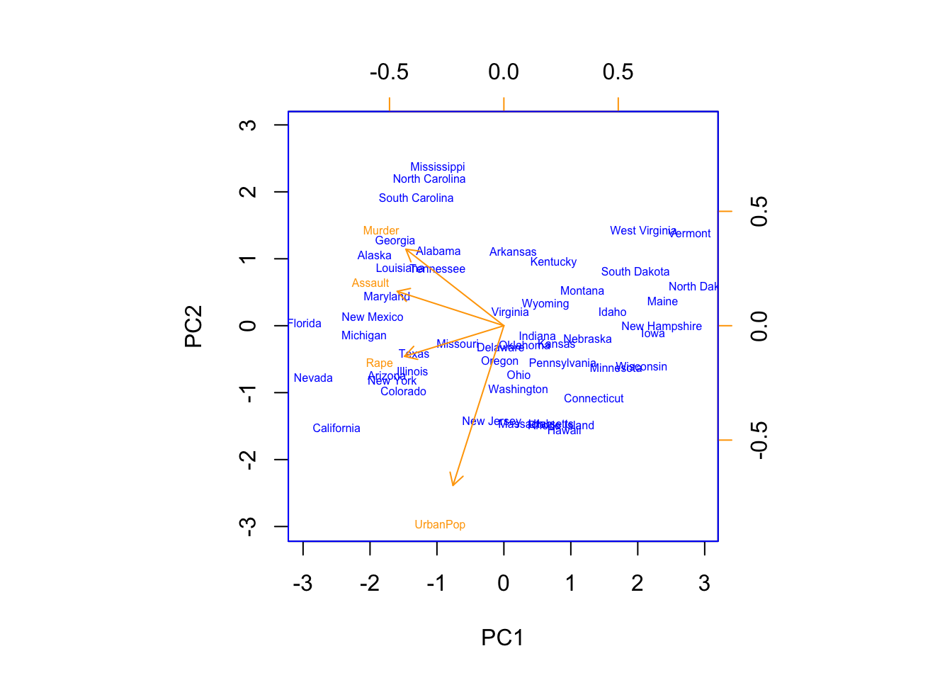

As will be discussed later, principal components are unique up to a sign change, so we can obtain the other identical possibility for the PC components by flipping the signs in both the rotation matrix i.e. PC scores (pr.out$rotation), and in the $\mathbf{X}$ matrix (pr.out$x).

To conclude the example, we’ll compute the PVE of each component. pr.out$sdev provides the standard deviations for each PC. So squaring each of these quanitites, and dividing by the sum of them provides the PVE explained by each principal component . Think about what the sd’s represent. Here, the 1st PC explains 62% of the variance, the second 25% and so on. We can plot the PVE explained by each component in a scree plot, and use the subjective criteria of when it elbows to determine the appropriate number of principal components.

pr.var <- pr.out$sdev^2
pve <- pr.var/sum(pr.var)
pve

## [1] 0.62006039 0.24744129 0.08914080 0.04335752

plot(pve, xlab="Principal Component",ylab = "PVE",
     ylim=c(0,1),type='b', main = "Scree Plot")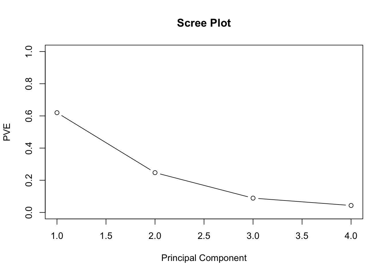

plot(cumsum(pve), xlab="Principal Component",ylab = "Cumulative PVE",
     ylim=c(0,1),type='b', main = "Cumulative PVE")

PCA-specific Considerations

Normalizing - Not only do variables have to be centered to mean zero, but their standard deviations needs to be scaled to 1, otherwise the magnitude of the loading vector (solution) will essentially be a consequence of the scale on which the variables were measured, and not the actual level of dispersion. There do exist some scenarios wheres scaling is not necessary, e.g. gene studies where variables share a measurement scale.

Uniqueness of PC’s - Both the loading and score vectors are unique up to a sign flip. Flip is irrelevant for the loading vector since the direction in p-dimensional space specified by each PC is unnaffected by a sign change (e.g. line intuition). Likewise, the score vectors are unique since the variances of $\mathbf{Z}$ is the same as variance of $\mathbf{-Z}$. Since $\mathbf{x_{ij}\approx \sum_{m=1}^M{z_{im}\phi_{jm}}}$. When $M=min(n-1,p)$, approximation is exact.

PVE - Projecting, for example, 3-dimensional data onto 2-dimensions sometimes reveals interesting patterns, e.g. clusters which could represent latent variables. One question is, “how much information is lost in projecting the data into a subspace, i.e. how much variance is not contained in the 1st few PC’s”? After centering, total variance present in a data set is defined as: \[ \sum_{j=1}^pVar(X_j) = \sum_{j=1}^p\frac1n\sum_{i=1}^nx_{ij}^2 \] and the variance of the m th PC is: \[ \frac1n\sum_{j=1}^pz_{im}^2 = \frac1n\sum_{j=1}^p(\sum_{i=1}^n\phi_{jm}x_{ij})^2 \] Therefore, the PVE of each PC is: \[ \frac{\frac1n\sum_{j=1}^p(\sum_{i=1}^n\phi_{jm}x_{ij})^2}{\sum_{j=1}^p\frac1n\sum_{i=1}^nx_{ij}^2} \] Thus, we can talk about variance explained in a specific PC, or cumulatively in the first m principal components.

How many PC’s - One solution is to examine where in the scree plot the line elbows, i.e. is noticably smaller from the previous one. Admittedly ad-hoc, but in defense, this analysis is exploratory.